Step 3: Transforming Data

The dplyr package (part of the tidyverse), aims to simplify the process of manipulating and transforming data in a straightforward and user-friendly manner. This is the second step in the tidyverse workflow.

A central principle of tidyverse packages, is the emphasis on minimizing the number of keystrokes and characters needed to attain desired results. In dplyr, the use of quotation marks for column names in data frames is often unnecessary. Another noteworthy aspect is that both the input to and output from all functions are in the form of data frames.

dplyr package offers a set of key functions, referred to as ‘verbs’, which can be combined to achieve specific and targeted outcomes. Users familiar with functions in Microsoft Excel may recognize similarities in the functionality provided by dplyr.

Before we delve into these functions in detail, let’s first explore filtering or subsetting data frames using base R functions.

Subsetting Data Frames

A frequently encountered task in data manipulation is filtering or subsetting data to a more focused and potentially relevant subset of values. Data frames (or tibbles) can be subset using base R functions.

Let’s start by reading the cms_hospital_patient_satisfaction_2016_sampled.csv into a data frame using the read_csv() function in readr package:

library(readr)
# here the first argument is a path
cms_data <- read_csv("data/cms_hospital_patient_satisfaction.csv")
# convert column names to R standard
library(janitor) # remember to install janitor: install.packages("janitor")
cms_data <- cms_data |> clean_names()

Subset by position

Here we use the [row, col] syntax to subset data frames.

To display a single value:

# display the value in 4th row and 2nd column
cms_data[4, 2]

Output

facility_name
MERCY HOSPITAL FORT SMITH

To display a single row: Here, the column value is omitted, thereby retrieving the entire column.

# display the 4th row
cms_data[4,]

Output

id	facility_name	county	hospital_type	star_rating	no_of_surveys	response_rate	overall_rating
040062	MERCY HOSPITAL FORT SMITH	SEBASTIAN	Acute Care Hospital	3	2506	35	3

To display a single column: (Note: columns can be given by name as well) Here, the row value is omitted, thereby retrieving the entire column.

# display the 3rd column
cms_data[, 3] # is same as cms_data[3]
# display the 3rd column (or County column)
cms_data[, "county"] # is same as cms_data["County"]

Output

county
SAN DIEGO
COOK
LAKE
SEBASTIAN
SHELBY
BRAZOS
GREENE
MONTEZUMA
VIRGINIA BEACH
FAYETTE
LOS ANGELES
MIAMI-DADE
SUMNER
ISLAND
LOS ANGELES

county
SAN DIEGO
COOK
LAKE
SEBASTIAN
SHELBY
BRAZOS
GREENE
MONTEZUMA
VIRGINIA BEACH
FAYETTE
LOS ANGELES
MIAMI-DADE
SUMNER
ISLAND
LOS ANGELES

To display a range of rows:

# using a vector of indexes
cms_data[c(3, 5, 1), ]
# subsetting
cms_data[2:4,]

Output

id	facility_name	county	hospital_type	star_rating	no_of_surveys	response_rate	overall_rating
100051	SOUTH LAKE HOSPITAL	LAKE	Acute Care Hospital	2	1382	20	2
440048	BAPTIST MEMORIAL HOSPITAL	SHELBY	Acute Care Hospital	2	1799	18	2
050424	SCRIPPS GREEN HOSPITAL	SAN DIEGO	Acute Care Hospital	4	3110	41	5

id	facility_name	county	hospital_type	star_rating	no_of_surveys	response_rate	overall_rating
140103	ST BERNARD HOSPITAL	COOK	Acute Care Hospital	1	264	6	2
100051	SOUTH LAKE HOSPITAL	LAKE	Acute Care Hospital	2	1382	20	2
040062	MERCY HOSPITAL FORT SMITH	SEBASTIAN	Acute Care Hospital	3	2506	35	3

To display a range of columns:

# using a vector of indexes
cms_data[, c(1, 3, 6), ]
# subsetting
cms_data[, 4:6]
# using a vector of column names
cms_data[, c("hospital_type", "overall_rating")]

Output

id	county	no_of_surveys
050424	SAN DIEGO	3110
140103	COOK	264
100051	LAKE	1382
040062	SEBASTIAN	2506
440048	SHELBY	1799
450011	BRAZOS	1379
151317	GREENE	114
061327	MONTEZUMA	247
490057	VIRGINIA BEACH	619
110215	FAYETTE	1714
050704	LOS ANGELES	241
100296	MIAMI-DADE	393
440003	SUMNER	680
501339	ISLAND	389
050116	LOS ANGELES	1110

hospital_type	star_rating	no_of_surveys
Acute Care Hospital	4	3110
Acute Care Hospital	1	264
Acute Care Hospital	2	1382
Acute Care Hospital	3	2506
Acute Care Hospital	2	1799
Acute Care Hospital	3	1379
Critical Access Hospital	3	114
Critical Access Hospital	4	247
Acute Care Hospital	4	619
Acute Care Hospital	2	1714
Acute Care Hospital	3	241
Acute Care Hospital	4	393
Acute Care Hospital	4	680
Critical Access Hospital	3	389
Acute Care Hospital	3	1110

hospital_type	overall_rating
Acute Care Hospital	5
Acute Care Hospital	2
Acute Care Hospital	2
Acute Care Hospital	3
Acute Care Hospital	2
Acute Care Hospital	3
Critical Access Hospital	3
Critical Access Hospital	3
Acute Care Hospital	3
Acute Care Hospital	2
Acute Care Hospital	3
Acute Care Hospital	3
Acute Care Hospital	2
Critical Access Hospital	3
Acute Care Hospital	2

To display multiple rows and columns:

cms_data[2:6, c("hospital_type", "no_of_surveys", "response_rate")]

Output

hospital_type	no_of_surveys	response_rate
Acute Care Hospital	264	6
Acute Care Hospital	1382	20
Acute Care Hospital	2506	35
Acute Care Hospital	1799	18
Acute Care Hospital	1379	24

To exclude a column (use -):

# display the data frame without Star_rating column
cms_data[-5]
# display the data frame, include only the hospital information and location
cms_data[c(-5, -6, -7, -8)] # or cms_data[c(1, 2, 3, 4)]

Output

id	facility_name	county	hospital_type	no_of_surveys	response_rate	overall_rating
050424	SCRIPPS GREEN HOSPITAL	SAN DIEGO	Acute Care Hospital	3110	41	5
140103	ST BERNARD HOSPITAL	COOK	Acute Care Hospital	264	6	2
100051	SOUTH LAKE HOSPITAL	LAKE	Acute Care Hospital	1382	20	2
040062	MERCY HOSPITAL FORT SMITH	SEBASTIAN	Acute Care Hospital	2506	35	3
440048	BAPTIST MEMORIAL HOSPITAL	SHELBY	Acute Care Hospital	1799	18	2
450011	ST JOSEPH REGIONAL HEALTH CENTER	BRAZOS	Acute Care Hospital	1379	24	3
151317	GREENE COUNTY GENERAL HOSPITAL	GREENE	Critical Access Hospital	114	22	3
061327	SOUTHWEST MEMORIAL HOSPITAL	MONTEZUMA	Critical Access Hospital	247	34	3
490057	SENTARA GENERAL HOSPITAL	VIRGINIA BEACH	Acute Care Hospital	619	32	3
110215	PIEDMONT FAYETTE HOSPITAL	FAYETTE	Acute Care Hospital	1714	21	2
050704	MISSION COMMUNITY HOSPITAL	LOS ANGELES	Acute Care Hospital	241	14	3
100296	DOCTORS HOSPITAL	MIAMI-DADE	Acute Care Hospital	393	24	3
440003	SUMNER REGIONAL MEDICAL CENTER	SUMNER	Acute Care Hospital	680	35	2
501339	WHIDBEY GENERAL HOSPITAL	ISLAND	Critical Access Hospital	389	29	3
050116	NORTHRIDGE MEDICAL CENTER	LOS ANGELES	Acute Care Hospital	1110	20	2

id	facility_name	county	hospital_type
050424	SCRIPPS GREEN HOSPITAL	SAN DIEGO	Acute Care Hospital
140103	ST BERNARD HOSPITAL	COOK	Acute Care Hospital
100051	SOUTH LAKE HOSPITAL	LAKE	Acute Care Hospital
040062	MERCY HOSPITAL FORT SMITH	SEBASTIAN	Acute Care Hospital
440048	BAPTIST MEMORIAL HOSPITAL	SHELBY	Acute Care Hospital
450011	ST JOSEPH REGIONAL HEALTH CENTER	BRAZOS	Acute Care Hospital
151317	GREENE COUNTY GENERAL HOSPITAL	GREENE	Critical Access Hospital
061327	SOUTHWEST MEMORIAL HOSPITAL	MONTEZUMA	Critical Access Hospital
490057	SENTARA GENERAL HOSPITAL	VIRGINIA BEACH	Acute Care Hospital
110215	PIEDMONT FAYETTE HOSPITAL	FAYETTE	Acute Care Hospital
050704	MISSION COMMUNITY HOSPITAL	LOS ANGELES	Acute Care Hospital
100296	DOCTORS HOSPITAL	MIAMI-DADE	Acute Care Hospital
440003	SUMNER REGIONAL MEDICAL CENTER	SUMNER	Acute Care Hospital
501339	WHIDBEY GENERAL HOSPITAL	ISLAND	Critical Access Hospital
050116	NORTHRIDGE MEDICAL CENTER	LOS ANGELES	Acute Care Hospital

Subset by condition

Apart from subsetting a vector based on the position of values, we can also ask questions about the set of values to R, and it will respond with TRUE or FALSE answers. This is often done using logical expressions to filter the data.

Which cells contain the value “LOS ANGELES”?

cms_data == "LOS ANGELES"

Output

         id facility_name county hospital_type star_rating no_of_surveys
 [1,] FALSE         FALSE  FALSE         FALSE       FALSE         FALSE
 [2,] FALSE         FALSE  FALSE         FALSE       FALSE         FALSE
 [3,] FALSE         FALSE  FALSE         FALSE       FALSE         FALSE
 [4,] FALSE         FALSE  FALSE         FALSE       FALSE         FALSE
 [5,] FALSE         FALSE  FALSE         FALSE       FALSE         FALSE
 [6,] FALSE         FALSE  FALSE         FALSE       FALSE         FALSE
 [7,] FALSE         FALSE  FALSE         FALSE       FALSE         FALSE
 [8,] FALSE         FALSE  FALSE         FALSE       FALSE         FALSE
 [9,] FALSE         FALSE  FALSE         FALSE       FALSE         FALSE
[10,] FALSE         FALSE  FALSE         FALSE       FALSE         FALSE
[11,] FALSE         FALSE   TRUE         FALSE       FALSE         FALSE
[12,] FALSE         FALSE  FALSE         FALSE       FALSE         FALSE
[13,] FALSE         FALSE  FALSE         FALSE       FALSE         FALSE
[14,] FALSE         FALSE  FALSE         FALSE       FALSE         FALSE
[15,] FALSE         FALSE   TRUE         FALSE       FALSE         FALSE
      response_rate overall_rating
 [1,]         FALSE          FALSE
 [2,]         FALSE          FALSE
 [3,]         FALSE          FALSE
 [4,]         FALSE          FALSE
 [5,]         FALSE          FALSE
 [6,]         FALSE          FALSE
 [7,]         FALSE          FALSE
 [8,]         FALSE          FALSE
 [9,]         FALSE          FALSE
[10,]         FALSE          FALSE
[11,]         FALSE          FALSE
[12,]         FALSE          FALSE
[13,]         FALSE          FALSE
[14,]         FALSE          FALSE
[15,]         FALSE          FALSE

R returns TRUE for values that satisfy the condition, and FALSE for those that don’t.

How many cells contain the word “LOS ANGELES”?

We can use the sum() function to compute the number of occurrences of “LOS ANGELES” in the data frame as it treats TRUE as 1 and FALSE as 0.

sum(cms_data == "LOS ANGELES")

Output

[1] 2

Which cells contain the value 3?

cms_data == 3

Output

         id facility_name county hospital_type star_rating no_of_surveys
 [1,] FALSE         FALSE  FALSE         FALSE       FALSE         FALSE
 [2,] FALSE         FALSE  FALSE         FALSE       FALSE         FALSE
 [3,] FALSE         FALSE  FALSE         FALSE       FALSE         FALSE
 [4,] FALSE         FALSE  FALSE         FALSE        TRUE         FALSE
 [5,] FALSE         FALSE  FALSE         FALSE       FALSE         FALSE
 [6,] FALSE         FALSE  FALSE         FALSE        TRUE         FALSE
 [7,] FALSE         FALSE  FALSE         FALSE        TRUE         FALSE
 [8,] FALSE         FALSE  FALSE         FALSE       FALSE         FALSE
 [9,] FALSE         FALSE  FALSE         FALSE       FALSE         FALSE
[10,] FALSE         FALSE  FALSE         FALSE       FALSE         FALSE
[11,] FALSE         FALSE  FALSE         FALSE        TRUE         FALSE
[12,] FALSE         FALSE  FALSE         FALSE       FALSE         FALSE
[13,] FALSE         FALSE  FALSE         FALSE       FALSE         FALSE
[14,] FALSE         FALSE  FALSE         FALSE        TRUE         FALSE
[15,] FALSE         FALSE  FALSE         FALSE        TRUE         FALSE
      response_rate overall_rating
 [1,]         FALSE          FALSE
 [2,]         FALSE          FALSE
 [3,]         FALSE          FALSE
 [4,]         FALSE           TRUE
 [5,]         FALSE          FALSE
 [6,]         FALSE           TRUE
 [7,]         FALSE           TRUE
 [8,]         FALSE           TRUE
 [9,]         FALSE           TRUE
[10,]         FALSE          FALSE
[11,]         FALSE           TRUE
[12,]         FALSE           TRUE
[13,]         FALSE          FALSE
[14,]         FALSE           TRUE
[15,]         FALSE          FALSE

We will use the comparison operators (see Section: Comparison Operators and Expressions) and logical operators (see Section: Logical Operators and Expressions) we explored in the subsequent sections.

Find all the facilities with a star rating above 3.

sr_above_3 <- cms_data$star_rating > 3
cms_data[sr_above_3, ]

Output

id	facility_name	county	hospital_type	star_rating	no_of_surveys	response_rate	overall_rating
050424	SCRIPPS GREEN HOSPITAL	SAN DIEGO	Acute Care Hospital	4	3110	41	5
061327	SOUTHWEST MEMORIAL HOSPITAL	MONTEZUMA	Critical Access Hospital	4	247	34	3
490057	SENTARA GENERAL HOSPITAL	VIRGINIA BEACH	Acute Care Hospital	4	619	32	3
100296	DOCTORS HOSPITAL	MIAMI-DADE	Acute Care Hospital	4	393	24	3
440003	SUMNER REGIONAL MEDICAL CENTER	SUMNER	Acute Care Hospital	4	680	35	2

Find all the facility names with a star rating above 2.

cms_data[sr_above_3, 2]

Output

facility_name
SCRIPPS GREEN HOSPITAL
SOUTHWEST MEMORIAL HOSPITAL
SENTARA GENERAL HOSPITAL
DOCTORS HOSPITAL
SUMNER REGIONAL MEDICAL CENTER

Find all the facilities with an overall rating of at least 3 and the response rate is above 30%.

# overall rating of at least 3
orate_aleast_3 <- cms_data["overall_rating"] >= 3
# response rate above 30\%
rrate_above_30 <- cms_data[7] > 30
# both conditions has to satisfy. hence and (&) operator
cms_data[(orate_aleast_3 & rrate_above_30), ]

Output

id	facility_name	county	hospital_type	star_rating	no_of_surveys	response_rate	overall_rating
050424	SCRIPPS GREEN HOSPITAL	SAN DIEGO	Acute Care Hospital	4	3110	41	5
040062	MERCY HOSPITAL FORT SMITH	SEBASTIAN	Acute Care Hospital	3	2506	35	3
061327	SOUTHWEST MEMORIAL HOSPITAL	MONTEZUMA	Critical Access Hospital	4	247	34	3
490057	SENTARA GENERAL HOSPITAL	VIRGINIA BEACH	Acute Care Hospital	4	619	32	3

# the above 3 commands can be combined into a single-line command
cms_data[(cms_data["overall_rating"] >= 3) & (cms_data[7] > 30), ]

Output

id	facility_name	county	hospital_type	star_rating	no_of_surveys	response_rate	overall_rating
050424	SCRIPPS GREEN HOSPITAL	SAN DIEGO	Acute Care Hospital	4	3110	41	5
040062	MERCY HOSPITAL FORT SMITH	SEBASTIAN	Acute Care Hospital	3	2506	35	3
061327	SOUTHWEST MEMORIAL HOSPITAL	MONTEZUMA	Critical Access Hospital	4	247	34	3
490057	SENTARA GENERAL HOSPITAL	VIRGINIA BEACH	Acute Care Hospital	4	619	32	3

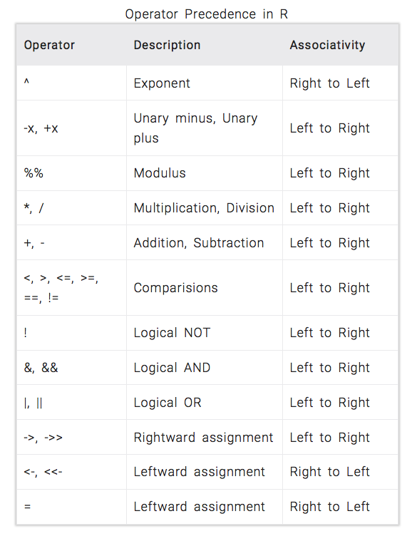
Operators in R have a specific precedence, and they are executed either from left $\rightarrow$ right or right $\rightarrow$ left. This can impact the expected result if you are not mindful of operator precedence. It is advisable to use parentheses to explicitly define the order of operations since parentheses have the highest precedence. Refer to this image for a operator precedence table.

For example: 5 + 3 * 2 is not the same as (5 + 3) * 2. The multiplication operation takes precedence over addition, potentially leading to unexpected results. Using parentheses ensures that the addition operation is performed first, providing the desired outcome.

Find the county of hospitals with any rating greater than or equal to 3.

# there are two ratings:
# 1. star_rating >= 3
srate_3 <- cms_data$star_rating >= 3
# 2. overall_rating >= 3
orate_3 <- cms_data["overall_rating"] >= 3
# any means at least one has to be >= 3 -> or operator
cms_data[srate_3 | orate_3, ]
# we only needs the county names
cms_data[srate_3 | orate_3, "county"]

Output

id	facility_name	county	hospital_type	star_rating	no_of_surveys	response_rate	overall_rating
050424	SCRIPPS GREEN HOSPITAL	SAN DIEGO	Acute Care Hospital	4	3110	41	5
040062	MERCY HOSPITAL FORT SMITH	SEBASTIAN	Acute Care Hospital	3	2506	35	3
450011	ST JOSEPH REGIONAL HEALTH CENTER	BRAZOS	Acute Care Hospital	3	1379	24	3
151317	GREENE COUNTY GENERAL HOSPITAL	GREENE	Critical Access Hospital	3	114	22	3
061327	SOUTHWEST MEMORIAL HOSPITAL	MONTEZUMA	Critical Access Hospital	4	247	34	3
490057	SENTARA GENERAL HOSPITAL	VIRGINIA BEACH	Acute Care Hospital	4	619	32	3
050704	MISSION COMMUNITY HOSPITAL	LOS ANGELES	Acute Care Hospital	3	241	14	3
100296	DOCTORS HOSPITAL	MIAMI-DADE	Acute Care Hospital	4	393	24	3
440003	SUMNER REGIONAL MEDICAL CENTER	SUMNER	Acute Care Hospital	4	680	35	2
501339	WHIDBEY GENERAL HOSPITAL	ISLAND	Critical Access Hospital	3	389	29	3
050116	NORTHRIDGE MEDICAL CENTER	LOS ANGELES	Acute Care Hospital	3	1110	20	2

county
SAN DIEGO
SEBASTIAN
BRAZOS
GREENE
MONTEZUMA
VIRGINIA BEACH
LOS ANGELES
MIAMI-DADE
SUMNER
ISLAND
LOS ANGELES

How many hospitals are categorized as Acute Care Hospital?

# all the hospitals categorized as Acute Care Hospitals 
hosp_acute <- cms_data$hospital_type == "Acute Care Hospital"
# summing the vector of TRUE (1) and FALSE (0) values 
sum(hosp_acute)

Output

[1] 12

Find the summary statistics number of surveys conducted at Critical Access Hospital.

# all the hospitals categorized as Critical Access Hospitals
hosp_crit <- cms_data$hospital_type == "Critical Access Hospital"
# number of surveys conducted in Critical Access Hospitals
nsurv_crit <- cms_data[hosp_crit, "no_of_surveys"]
# summary statistics of the number of surveys
summary(nsurv_crit)

Output

 no_of_surveys  
 Min.   :114.0  
 1st Qu.:180.5  
 Median :247.0  
 Mean   :250.0  
 3rd Qu.:318.0  
 Max.   :389.0

This approach can be somewhat cumbersome. It requires repeated referencing of the data frame name, leading to a multiple use of punctuation that needs careful management. In the following section, we will leverage the dplyrpackage and its functions to craft more concise code, and efficient data manipulations.

Data manipulation with `dplyr’ functions

You’ll primarily use six key dplyr functions for data manipulations:

filter(): pick observations based on their values.
select(): pick variables by their names.
mutate(): create new variables using functions applied to existing variables.
summarise(): collapse multiple values into a single summary.
group_by(): group the rows based on specified criteria.
arrange(): reorder the rows based on specified criteria.

If you’ve already installed the tidyverse package (if not, you can do so by running the command: install.packages("tidyverse")), let’s proceed to load it into our R session first:

library(tidyverse)

`filter()`

The filter() function takes logical expressions and returns the rows for which all are TRUE.

Example 1: Filter the cms_data data frame to find all the facilities with an overall_rating of 3.

cms_data |> filter(overall_rating == 3)

Output

id	facility_name	county	hospital_type	star_rating	no_of_surveys	response_rate	overall_rating
040062	MERCY HOSPITAL FORT SMITH	SEBASTIAN	Acute Care Hospital	3	2506	35	3
450011	ST JOSEPH REGIONAL HEALTH CENTER	BRAZOS	Acute Care Hospital	3	1379	24	3
151317	GREENE COUNTY GENERAL HOSPITAL	GREENE	Critical Access Hospital	3	114	22	3
061327	SOUTHWEST MEMORIAL HOSPITAL	MONTEZUMA	Critical Access Hospital	4	247	34	3
490057	SENTARA GENERAL HOSPITAL	VIRGINIA BEACH	Acute Care Hospital	4	619	32	3
050704	MISSION COMMUNITY HOSPITAL	LOS ANGELES	Acute Care Hospital	3	241	14	3
100296	DOCTORS HOSPITAL	MIAMI-DADE	Acute Care Hospital	4	393	24	3
501339	WHIDBEY GENERAL HOSPITAL	ISLAND	Critical Access Hospital	3	389	29	3

Here we are sending the cms_data data frame into the function filter() which tests each value in overall_rating column for the value 3 and returns the rows where this condition is TRUE.

You can check the dimension (number of rows and number of columns) of the resulting data frame by sending into the dim() function as follows:

cms_data |> filter(overall_rating == 3) |> dim()

Output

[1] 8 8

Example 2: Find all the facilities categorized as “Acute Care Hospital”. Here we filter on character data.

cms_data |> filter(hospital_type == "Acute Care Hospital")

Output

id	facility_name	county	hospital_type	star_rating	no_of_surveys	response_rate	overall_rating
050424	SCRIPPS GREEN HOSPITAL	SAN DIEGO	Acute Care Hospital	4	3110	41	5
140103	ST BERNARD HOSPITAL	COOK	Acute Care Hospital	1	264	6	2
100051	SOUTH LAKE HOSPITAL	LAKE	Acute Care Hospital	2	1382	20	2
040062	MERCY HOSPITAL FORT SMITH	SEBASTIAN	Acute Care Hospital	3	2506	35	3
440048	BAPTIST MEMORIAL HOSPITAL	SHELBY	Acute Care Hospital	2	1799	18	2
450011	ST JOSEPH REGIONAL HEALTH CENTER	BRAZOS	Acute Care Hospital	3	1379	24	3
490057	SENTARA GENERAL HOSPITAL	VIRGINIA BEACH	Acute Care Hospital	4	619	32	3
110215	PIEDMONT FAYETTE HOSPITAL	FAYETTE	Acute Care Hospital	2	1714	21	2
050704	MISSION COMMUNITY HOSPITAL	LOS ANGELES	Acute Care Hospital	3	241	14	3
100296	DOCTORS HOSPITAL	MIAMI-DADE	Acute Care Hospital	4	393	24	3
440003	SUMNER REGIONAL MEDICAL CENTER	SUMNER	Acute Care Hospital	4	680	35	2
050116	NORTHRIDGE MEDICAL CENTER	LOS ANGELES	Acute Care Hospital	3	1110	20	2

We can use logical operators introduced before to combine multiple conditions as follows.

Example 3: Find all the facilities categorized as “Acute Care Hospital” and has a overall rating of above 3.

cms_data |> filter(hospital_type == "Acute Care Hospital" & overall_rating > 3)

Output

id	facility_name	county	hospital_type	star_rating	no_of_surveys	response_rate	overall_rating
050424	SCRIPPS GREEN HOSPITAL	SAN DIEGO	Acute Care Hospital	4	3110	41	5

Example 4: Find the facilities with any rating greater than or equal to 3.

cms_data |> filter(star_rating >= 3 | overall_rating >= 3)

Output

id	facility_name	county	hospital_type	star_rating	no_of_surveys	response_rate	overall_rating
050424	SCRIPPS GREEN HOSPITAL	SAN DIEGO	Acute Care Hospital	4	3110	41	5
040062	MERCY HOSPITAL FORT SMITH	SEBASTIAN	Acute Care Hospital	3	2506	35	3
450011	ST JOSEPH REGIONAL HEALTH CENTER	BRAZOS	Acute Care Hospital	3	1379	24	3
151317	GREENE COUNTY GENERAL HOSPITAL	GREENE	Critical Access Hospital	3	114	22	3
061327	SOUTHWEST MEMORIAL HOSPITAL	MONTEZUMA	Critical Access Hospital	4	247	34	3
490057	SENTARA GENERAL HOSPITAL	VIRGINIA BEACH	Acute Care Hospital	4	619	32	3
050704	MISSION COMMUNITY HOSPITAL	LOS ANGELES	Acute Care Hospital	3	241	14	3
100296	DOCTORS HOSPITAL	MIAMI-DADE	Acute Care Hospital	4	393	24	3
440003	SUMNER REGIONAL MEDICAL CENTER	SUMNER	Acute Care Hospital	4	680	35	2
501339	WHIDBEY GENERAL HOSPITAL	ISLAND	Critical Access Hospital	3	389	29	3
050116	NORTHRIDGE MEDICAL CENTER	LOS ANGELES	Acute Care Hospital	3	1110	20	2

Example 5: Find the facilitites with any rating greater than or equal to 3 and the response rate is above 30.

cms_data |> filter(star_rating >= 3 | overall_rating >= 3 & response_rate > 30)

Output

id	facility_name	county	hospital_type	star_rating	no_of_surveys	response_rate	overall_rating
050424	SCRIPPS GREEN HOSPITAL	SAN DIEGO	Acute Care Hospital	4	3110	41	5
040062	MERCY HOSPITAL FORT SMITH	SEBASTIAN	Acute Care Hospital	3	2506	35	3
450011	ST JOSEPH REGIONAL HEALTH CENTER	BRAZOS	Acute Care Hospital	3	1379	24	3
151317	GREENE COUNTY GENERAL HOSPITAL	GREENE	Critical Access Hospital	3	114	22	3
061327	SOUTHWEST MEMORIAL HOSPITAL	MONTEZUMA	Critical Access Hospital	4	247	34	3
490057	SENTARA GENERAL HOSPITAL	VIRGINIA BEACH	Acute Care Hospital	4	619	32	3
050704	MISSION COMMUNITY HOSPITAL	LOS ANGELES	Acute Care Hospital	3	241	14	3
100296	DOCTORS HOSPITAL	MIAMI-DADE	Acute Care Hospital	4	393	24	3
440003	SUMNER REGIONAL MEDICAL CENTER	SUMNER	Acute Care Hospital	4	680	35	2
501339	WHIDBEY GENERAL HOSPITAL	ISLAND	Critical Access Hospital	3	389	29	3
050116	NORTHRIDGE MEDICAL CENTER	LOS ANGELES	Acute Care Hospital	3	1110	20	2

The output of the above command is incorrect. Recall R operator precedence where & operator precedes | operator. Therefore, the command overall_rating >= 3 & response_rate > 30 is evaluated first. This can be verified by adding brackets around this command as follows: To fix the issue add brackets as follows:

cms_data |> filter(star_rating >= 3 | (overall_rating >= 3 & response_rate > 30))

Output

id	facility_name	county	hospital_type	star_rating	no_of_surveys	response_rate	overall_rating
050424	SCRIPPS GREEN HOSPITAL	SAN DIEGO	Acute Care Hospital	4	3110	41	5
040062	MERCY HOSPITAL FORT SMITH	SEBASTIAN	Acute Care Hospital	3	2506	35	3
450011	ST JOSEPH REGIONAL HEALTH CENTER	BRAZOS	Acute Care Hospital	3	1379	24	3
151317	GREENE COUNTY GENERAL HOSPITAL	GREENE	Critical Access Hospital	3	114	22	3
061327	SOUTHWEST MEMORIAL HOSPITAL	MONTEZUMA	Critical Access Hospital	4	247	34	3
490057	SENTARA GENERAL HOSPITAL	VIRGINIA BEACH	Acute Care Hospital	4	619	32	3
050704	MISSION COMMUNITY HOSPITAL	LOS ANGELES	Acute Care Hospital	3	241	14	3
100296	DOCTORS HOSPITAL	MIAMI-DADE	Acute Care Hospital	4	393	24	3
440003	SUMNER REGIONAL MEDICAL CENTER	SUMNER	Acute Care Hospital	4	680	35	2
501339	WHIDBEY GENERAL HOSPITAL	ISLAND	Critical Access Hospital	3	389	29	3
050116	NORTHRIDGE MEDICAL CENTER	LOS ANGELES	Acute Care Hospital	3	1110	20	2

To fix the issue add brackets as follows:

cms_data |> filter((star_rating >= 3 | overall_rating >= 3) & response_rate > 30)

Output

id	facility_name	county	hospital_type	star_rating	no_of_surveys	response_rate	overall_rating
050424	SCRIPPS GREEN HOSPITAL	SAN DIEGO	Acute Care Hospital	4	3110	41	5
040062	MERCY HOSPITAL FORT SMITH	SEBASTIAN	Acute Care Hospital	3	2506	35	3
061327	SOUTHWEST MEMORIAL HOSPITAL	MONTEZUMA	Critical Access Hospital	4	247	34	3
490057	SENTARA GENERAL HOSPITAL	VIRGINIA BEACH	Acute Care Hospital	4	619	32	3
440003	SUMNER REGIONAL MEDICAL CENTER	SUMNER	Acute Care Hospital	4	680	35	2

This results in the correct output.

`%in%` helper

The %in% function is used to determine whether elements of one vector are present in another vector. It returns a logical vector indicating whether each element of the first vector is found in the second vector.

When we want to filter a subset of rows that may contain multiple different values, it’s more efficient to provide a vector of the values of interest instead of combining multiple OR commands.

Example 6: Retrieve a subset of facilities that have an odd number of overall rating.

cms_data |> filter(overall_rating %in% c(1, 3, 5))

Output

id	facility_name	county	hospital_type	star_rating	no_of_surveys	response_rate	overall_rating
050424	SCRIPPS GREEN HOSPITAL	SAN DIEGO	Acute Care Hospital	4	3110	41	5
040062	MERCY HOSPITAL FORT SMITH	SEBASTIAN	Acute Care Hospital	3	2506	35	3
450011	ST JOSEPH REGIONAL HEALTH CENTER	BRAZOS	Acute Care Hospital	3	1379	24	3
151317	GREENE COUNTY GENERAL HOSPITAL	GREENE	Critical Access Hospital	3	114	22	3
061327	SOUTHWEST MEMORIAL HOSPITAL	MONTEZUMA	Critical Access Hospital	4	247	34	3
490057	SENTARA GENERAL HOSPITAL	VIRGINIA BEACH	Acute Care Hospital	4	619	32	3
050704	MISSION COMMUNITY HOSPITAL	LOS ANGELES	Acute Care Hospital	3	241	14	3
100296	DOCTORS HOSPITAL	MIAMI-DADE	Acute Care Hospital	4	393	24	3
501339	WHIDBEY GENERAL HOSPITAL	ISLAND	Critical Access Hospital	3	389	29	3

`str_detect` function

The str_detect() function is part of the stringr package and is used for pattern matching within strings. It allows you to search for a specific pattern or regular expression (discussed later) within a character vector or string.

Example 1: Find all the facilities that contains GENERAL in their name from the cms_data data frame.

cms_data |> filter(
  str_detect(facility_name, 'GENERAL')
  )

Output

id	facility_name	county	hospital_type	star_rating	no_of_surveys	response_rate	overall_rating
151317	GREENE COUNTY GENERAL HOSPITAL	GREENE	Critical Access Hospital	3	114	22	3
490057	SENTARA GENERAL HOSPITAL	VIRGINIA BEACH	Acute Care Hospital	4	619	32	3
501339	WHIDBEY GENERAL HOSPITAL	ISLAND	Critical Access Hospital	3	389	29	3

`select()`

The select() function returns a subset of the variables or columns.

This function can accept column names (even without quotation marks) or the column position number starting from the left. Unlike in base R (we explore before), commands within the brackets in select() do not need to be concatenated using c().

Example 1: Extract the facility name, hospital type and overall rating columns from cms_data data frame.

cms_data |> select(facility_name, hospital_type, overall_rating)

Output

facility_name	hospital_type	overall_rating
SCRIPPS GREEN HOSPITAL	Acute Care Hospital	5
ST BERNARD HOSPITAL	Acute Care Hospital	2
SOUTH LAKE HOSPITAL	Acute Care Hospital	2
MERCY HOSPITAL FORT SMITH	Acute Care Hospital	3
BAPTIST MEMORIAL HOSPITAL	Acute Care Hospital	2
ST JOSEPH REGIONAL HEALTH CENTER	Acute Care Hospital	3
GREENE COUNTY GENERAL HOSPITAL	Critical Access Hospital	3
SOUTHWEST MEMORIAL HOSPITAL	Critical Access Hospital	3
SENTARA GENERAL HOSPITAL	Acute Care Hospital	3
PIEDMONT FAYETTE HOSPITAL	Acute Care Hospital	2
MISSION COMMUNITY HOSPITAL	Acute Care Hospital	3
DOCTORS HOSPITAL	Acute Care Hospital	3
SUMNER REGIONAL MEDICAL CENTER	Acute Care Hospital	2
WHIDBEY GENERAL HOSPITAL	Critical Access Hospital	3
NORTHRIDGE MEDICAL CENTER	Acute Care Hospital	2

Using column positions:

cms_data |> select(2, 4, 8)

Output

facility_name	hospital_type	overall_rating
SCRIPPS GREEN HOSPITAL	Acute Care Hospital	5
ST BERNARD HOSPITAL	Acute Care Hospital	2
SOUTH LAKE HOSPITAL	Acute Care Hospital	2
MERCY HOSPITAL FORT SMITH	Acute Care Hospital	3
BAPTIST MEMORIAL HOSPITAL	Acute Care Hospital	2
ST JOSEPH REGIONAL HEALTH CENTER	Acute Care Hospital	3
GREENE COUNTY GENERAL HOSPITAL	Critical Access Hospital	3
SOUTHWEST MEMORIAL HOSPITAL	Critical Access Hospital	3
SENTARA GENERAL HOSPITAL	Acute Care Hospital	3
PIEDMONT FAYETTE HOSPITAL	Acute Care Hospital	2
MISSION COMMUNITY HOSPITAL	Acute Care Hospital	3
DOCTORS HOSPITAL	Acute Care Hospital	3
SUMNER REGIONAL MEDICAL CENTER	Acute Care Hospital	2
WHIDBEY GENERAL HOSPITAL	Critical Access Hospital	3
NORTHRIDGE MEDICAL CENTER	Acute Care Hospital	2

We can use the ‘-’ symbol to extract all columns except for specific ones:

cms_data |> dplyr::select(-id, -county_name, -star_rating, -no_of_surveys, -response_rate)

Output

facility_name	hospital_type	overall_rating
SCRIPPS GREEN HOSPITAL	Acute Care Hospital	5
ST BERNARD HOSPITAL	Acute Care Hospital	2
SOUTH LAKE HOSPITAL	Acute Care Hospital	2
MERCY HOSPITAL FORT SMITH	Acute Care Hospital	3
BAPTIST MEMORIAL HOSPITAL	Acute Care Hospital	2
ST JOSEPH REGIONAL HEALTH CENTER	Acute Care Hospital	3
GREENE COUNTY GENERAL HOSPITAL	Critical Access Hospital	3
SOUTHWEST MEMORIAL HOSPITAL	Critical Access Hospital	3
SENTARA GENERAL HOSPITAL	Acute Care Hospital	3
PIEDMONT FAYETTE HOSPITAL	Acute Care Hospital	2
MISSION COMMUNITY HOSPITAL	Acute Care Hospital	3
DOCTORS HOSPITAL	Acute Care Hospital	3
SUMNER REGIONAL MEDICAL CENTER	Acute Care Hospital	2
WHIDBEY GENERAL HOSPITAL	Critical Access Hospital	3
NORTHRIDGE MEDICAL CENTER	Acute Care Hospital	2

Or use a combination of column names and positions:

cms_data |> select(2, 4, overall_rating)

Output

facility_name	hospital_type	overall_rating
SCRIPPS GREEN HOSPITAL	Acute Care Hospital	5
ST BERNARD HOSPITAL	Acute Care Hospital	2
SOUTH LAKE HOSPITAL	Acute Care Hospital	2
MERCY HOSPITAL FORT SMITH	Acute Care Hospital	3
BAPTIST MEMORIAL HOSPITAL	Acute Care Hospital	2
ST JOSEPH REGIONAL HEALTH CENTER	Acute Care Hospital	3
GREENE COUNTY GENERAL HOSPITAL	Critical Access Hospital	3
SOUTHWEST MEMORIAL HOSPITAL	Critical Access Hospital	3
SENTARA GENERAL HOSPITAL	Acute Care Hospital	3
PIEDMONT FAYETTE HOSPITAL	Acute Care Hospital	2
MISSION COMMUNITY HOSPITAL	Acute Care Hospital	3
DOCTORS HOSPITAL	Acute Care Hospital	3
SUMNER REGIONAL MEDICAL CENTER	Acute Care Hospital	2
WHIDBEY GENERAL HOSPITAL	Critical Access Hospital	3
NORTHRIDGE MEDICAL CENTER	Acute Care Hospital	2

Useful helper functions

The select helper functions (check ?select_helpers) are a set of convenience functions provided by the dplyr package. These functions offer shortcuts for selecting columns based on specific criteria or patterns, making it easier to work with data frames.

Some commonly used select helper functions include:

starts_with(): selects columns that start with a specified prefix.

cms_data |> select(starts_with('s'))

Output

star_rating
4
1
2
3
2
3
3
4
4
2
3
4
4
3
3

ends_with(): selects columns that end with a specified suffix.

cms_data |> select(ends_with('g'))

Output

star_rating	overall_rating
4	5
1	2
2	2
3	3
2	2
3	3
3	3
4	3
4	3
2	2
3	3
4	3
4	2
3	3
3	2

contains(): selects columns that contain a specified substring.

cms_data |> select(contains('name'))

Output

facility_name
SCRIPPS GREEN HOSPITAL
ST BERNARD HOSPITAL
SOUTH LAKE HOSPITAL
MERCY HOSPITAL FORT SMITH
BAPTIST MEMORIAL HOSPITAL
ST JOSEPH REGIONAL HEALTH CENTER
GREENE COUNTY GENERAL HOSPITAL
SOUTHWEST MEMORIAL HOSPITAL
SENTARA GENERAL HOSPITAL
PIEDMONT FAYETTE HOSPITAL
MISSION COMMUNITY HOSPITAL
DOCTORS HOSPITAL
SUMNER REGIONAL MEDICAL CENTER
WHIDBEY GENERAL HOSPITAL
NORTHRIDGE MEDICAL CENTER

cms_data |> select(contains('f'))

Output

facility_name	no_of_surveys
SCRIPPS GREEN HOSPITAL	3110
ST BERNARD HOSPITAL	264
SOUTH LAKE HOSPITAL	1382
MERCY HOSPITAL FORT SMITH	2506
BAPTIST MEMORIAL HOSPITAL	1799
ST JOSEPH REGIONAL HEALTH CENTER	1379
GREENE COUNTY GENERAL HOSPITAL	114
SOUTHWEST MEMORIAL HOSPITAL	247
SENTARA GENERAL HOSPITAL	619
PIEDMONT FAYETTE HOSPITAL	1714
MISSION COMMUNITY HOSPITAL	241
DOCTORS HOSPITAL	393
SUMNER REGIONAL MEDICAL CENTER	680
WHIDBEY GENERAL HOSPITAL	389
NORTHRIDGE MEDICAL CENTER	1110

matches(): selects columns that match a specified regular expression pattern.

cms_data |> select(
  matches('[a-z]_[a-z]{4}$')
  )

Output

facility_name	hospital_type	response_rate
SCRIPPS GREEN HOSPITAL	Acute Care Hospital	41
ST BERNARD HOSPITAL	Acute Care Hospital	6
SOUTH LAKE HOSPITAL	Acute Care Hospital	20
MERCY HOSPITAL FORT SMITH	Acute Care Hospital	35
BAPTIST MEMORIAL HOSPITAL	Acute Care Hospital	18
ST JOSEPH REGIONAL HEALTH CENTER	Acute Care Hospital	24
GREENE COUNTY GENERAL HOSPITAL	Critical Access Hospital	22
SOUTHWEST MEMORIAL HOSPITAL	Critical Access Hospital	34
SENTARA GENERAL HOSPITAL	Acute Care Hospital	32
PIEDMONT FAYETTE HOSPITAL	Acute Care Hospital	21
MISSION COMMUNITY HOSPITAL	Acute Care Hospital	14
DOCTORS HOSPITAL	Acute Care Hospital	24
SUMNER REGIONAL MEDICAL CENTER	Acute Care Hospital	35
WHIDBEY GENERAL HOSPITAL	Critical Access Hospital	29
NORTHRIDGE MEDICAL CENTER	Acute Care Hospital	20

Here, the regular expression [a-z]_[a-z]{4}$ can be broken down into smaller chunks for better understanding:

[a-z] matches a set of lowercase characters from ‘a’ to ‘z’.
_ matches an underscore.
[a-z]{4} matches any four lowercase characters from ‘a’ to ‘z’.

Putting this together, the expression selects column names that have four characters after an underscore. Thus, it should match column names: facility_name, county_name, hospital_type, and response_rate.

If you’re unfamiliar with regular expressions, you can skip this section for now. However, interested readers can find many online resources to learn about regular expressions. One of my favorite online tools for building and testing regular expressions is https://regexr.com. You can use this tool to test the correctness of a regular expression.

num_range(): selects columns based on a numeric range.

Let’s use the count data frame for this example. First read the csv file: GSE60450_normalized_data.csv.

counts <- read_csv("data/GSE60450_normalized_data.csv")
colnames(counts)

Output

Rows: 20 Columns: 14
── Column specification ────────────────────────────────────────────────────────
Delimiter: ","
chr  (2): X, gene_symbol
dbl (12): GSM1480291, GSM1480292, GSM1480293, GSM1480294, GSM1480295, GSM148...

ℹ Use `spec()` to retrieve the full column specification for this data.
ℹ Specify the column types or set `show_col_types = FALSE` to quiet this message.

 [1] "X"           "gene_symbol" "GSM1480291"  "GSM1480292"  "GSM1480293" 
 [6] "GSM1480294"  "GSM1480295"  "GSM1480296"  "GSM1480297"  "GSM1480298" 
[11] "GSM1480299"  "GSM1480300"  "GSM1480301"  "GSM1480302"

To select the samples from GSM1480297 to GSM1480300:

counts |> select(
  num_range(prefix = "GSM1480", 297:300)
  )

Output

GSM1480297	GSM1480298	GSM1480299	GSM1480300
10.59006	14.88337	7.57182	7.05763
95.67017	100.73912	78.07470	59.35009
0.00000	0.00000	0.00000	0.00000
125.00263	102.99289	110.64124	97.98130
0.00000	0.08505	0.07726	0.08255
33.84822	36.91075	27.46715	31.36722
0.00000	0.00000	0.00000	0.00000
281.97525	241.83343	227.84988	232.81909
62.62120	61.82975	49.98944	42.01557
17.98312	13.69270	9.00119	9.69908
51.79137	49.49782	52.84819	47.00956
50.07299	50.94364	45.04458	36.89776
147.58143	128.20957	168.08661	133.35197
52.83040	84.66509	323.54064	485.86178
0.07992	0.00000	0.00000	0.00000
0.00000	0.00000	0.03863	0.00000
102.26398	81.05056	115.31568	138.38724
0.03996	0.00000	0.00000	0.00000
0.00000	0.00000	0.00000	0.00000
14.02683	11.56650	12.13036	12.21671

all_of(): selects columns specified by character vector.

cms_data |> select(
  all_of(c("star_rating", "no_of_surveys", "response_rate", "no_column_by_this_name"))
  )

Error in `all_of()`:
! Can't subset columns that don't exist.
✖ Column `no_column_by_this_name` doesn't exist.

When using all_of(), all the names provided by the vector must be present in the data frame. Otherwise, it will result in an error, as shown above.

cms_data |> select(
  all_of(c("star_rating", "no_of_surveys", "response_rate"))
  )

Output

star_rating	no_of_surveys	response_rate
4	3110	41
1	264	6
2	1382	20
3	2506	35
2	1799	18
3	1379	24
3	114	22
4	247	34
4	619	32
2	1714	21
3	241	14
4	393	24
4	680	35
3	389	29
3	1110	20

any_of(): selects columns specified by character vector, allowing any of them to be present.

cms_data |> select(
  any_of(c("star_rating", "no_of_surveys", "response_rate", "no_column_by_this_name"))
  )

Output

star_rating	no_of_surveys	response_rate
4	3110	41
1	264	6
2	1382	20
3	2506	35
2	1799	18
3	1379	24
3	114	22
4	247	34
4	619	32
2	1714	21
3	241	14
4	393	24
4	680	35
3	389	29
3	1110	20

everything(): Selects all columns.

This function returns all column names that have not been specified. It is often used when reordering all columns in a dataframe:

cms_data |> select(5, 8, 2, everything())

Output

star_rating	overall_rating	facility_name	id	county	hospital_type	no_of_surveys	response_rate
4	5	SCRIPPS GREEN HOSPITAL	050424	SAN DIEGO	Acute Care Hospital	3110	41
1	2	ST BERNARD HOSPITAL	140103	COOK	Acute Care Hospital	264	6
2	2	SOUTH LAKE HOSPITAL	100051	LAKE	Acute Care Hospital	1382	20
3	3	MERCY HOSPITAL FORT SMITH	040062	SEBASTIAN	Acute Care Hospital	2506	35
2	2	BAPTIST MEMORIAL HOSPITAL	440048	SHELBY	Acute Care Hospital	1799	18
3	3	ST JOSEPH REGIONAL HEALTH CENTER	450011	BRAZOS	Acute Care Hospital	1379	24
3	3	GREENE COUNTY GENERAL HOSPITAL	151317	GREENE	Critical Access Hospital	114	22
4	3	SOUTHWEST MEMORIAL HOSPITAL	061327	MONTEZUMA	Critical Access Hospital	247	34
4	3	SENTARA GENERAL HOSPITAL	490057	VIRGINIA BEACH	Acute Care Hospital	619	32
2	2	PIEDMONT FAYETTE HOSPITAL	110215	FAYETTE	Acute Care Hospital	1714	21
3	3	MISSION COMMUNITY HOSPITAL	050704	LOS ANGELES	Acute Care Hospital	241	14
4	3	DOCTORS HOSPITAL	100296	MIAMI-DADE	Acute Care Hospital	393	24
4	2	SUMNER REGIONAL MEDICAL CENTER	440003	SUMNER	Acute Care Hospital	680	35
3	3	WHIDBEY GENERAL HOSPITAL	501339	ISLAND	Critical Access Hospital	389	29
3	2	NORTHRIDGE MEDICAL CENTER	050116	LOS ANGELES	Acute Care Hospital	1110	20

Here the dimensions of the dataframe is not changed, merely the column order.

You can combine multiple helper functions to create more complex selection criteria. Additionally, you can use the ‘-’ symbol in front of the helper function to exclude the matched columns.

For example try the following examples:

cms_data |> select(starts_with('i'), contains('rating'))
cms_data |> select(ends_with("type"), everything(), -1, -3)

`mutate()`

The mutate() function adds new columns of data, thus ‘mutating’ the contents and dimensions of the input data frame.

Example 1: Calculate the total number of patients or visitors who responded to the survey in each facility (i.e, $\text{response rate } = \frac{\text{number of responses}}{\text{total number of surveys}} \times 100$).

Here we use the round() function to round off the result to the closest integer or numeric value as number of responses cannot contain decimal values.

cms_data |> 
  mutate(no_of_responses = round(no_of_surveys * response_rate / 100))

Output

id	facility_name	county	hospital_type	star_rating	no_of_surveys	response_rate	overall_rating	no_of_responses
050424	SCRIPPS GREEN HOSPITAL	SAN DIEGO	Acute Care Hospital	4	3110	41	5	127510
140103	ST BERNARD HOSPITAL	COOK	Acute Care Hospital	1	264	6	2	1584
100051	SOUTH LAKE HOSPITAL	LAKE	Acute Care Hospital	2	1382	20	2	27640
040062	MERCY HOSPITAL FORT SMITH	SEBASTIAN	Acute Care Hospital	3	2506	35	3	87710
440048	BAPTIST MEMORIAL HOSPITAL	SHELBY	Acute Care Hospital	2	1799	18	2	32382
450011	ST JOSEPH REGIONAL HEALTH CENTER	BRAZOS	Acute Care Hospital	3	1379	24	3	33096
151317	GREENE COUNTY GENERAL HOSPITAL	GREENE	Critical Access Hospital	3	114	22	3	2508
061327	SOUTHWEST MEMORIAL HOSPITAL	MONTEZUMA	Critical Access Hospital	4	247	34	3	8398
490057	SENTARA GENERAL HOSPITAL	VIRGINIA BEACH	Acute Care Hospital	4	619	32	3	19808
110215	PIEDMONT FAYETTE HOSPITAL	FAYETTE	Acute Care Hospital	2	1714	21	2	35994
050704	MISSION COMMUNITY HOSPITAL	LOS ANGELES	Acute Care Hospital	3	241	14	3	3374
100296	DOCTORS HOSPITAL	MIAMI-DADE	Acute Care Hospital	4	393	24	3	9432
440003	SUMNER REGIONAL MEDICAL CENTER	SUMNER	Acute Care Hospital	4	680	35	2	23800
501339	WHIDBEY GENERAL HOSPITAL	ISLAND	Critical Access Hospital	3	389	29	3	11281
050116	NORTHRIDGE MEDICAL CENTER	LOS ANGELES	Acute Care Hospital	3	1110	20	2	22200

This creates a new column at the end of the data frame named ‘no_of_responses’ and computes the total number of responses. Because the number of columns is expanding, we can reduce the number of columns displayed using the select() function.

To do this, we need to use chaining which is discussed below.

Chaining functions

R chaining allows you to streamline your data analysis workflow by sequentially applying multiple operations to your data using the pipe operator |>. We often need to perform several data manipulation or analysis operations in a sequence. Chaining allows you to apply these operations one after the other in a clear and concise manner.

Here’s a basic template for chaining operations using the pipe operator |>:

result <- data |>
    operation1(...) |>
    operation2(...) |>
    operation3(...) |>
    ...
    operationN(...)

In this template:

data represents the input data frame or object.
operation1, operation2, …, operationN represent the functions or operations you want to apply sequentially to the data.For example: select(), filter() or mutate() functions.
... represents any additional arguments or parameters that may be passed to each operation.

Each operation takes the output of the previous operation as its input, making it easy to chain multiple operations together. This improves the readability of your code by organizing operations in a left-to-right fashion and it avoids creating intermediate variables to store the results of each operation.

`mutate()` continued

Let’s use chaining to combine both select() and mutate() operations for the previos example:

cms_data |> 
  select(facility_name, no_of_surveys, response_rate) |> 
  mutate(no_of_responses = round(no_of_surveys * response_rate / 100))

Output

facility_name	no_of_surveys	response_rate	no_of_responses
SCRIPPS GREEN HOSPITAL	3110	41	127510
ST BERNARD HOSPITAL	264	6	1584
SOUTH LAKE HOSPITAL	1382	20	27640
MERCY HOSPITAL FORT SMITH	2506	35	87710
BAPTIST MEMORIAL HOSPITAL	1799	18	32382
ST JOSEPH REGIONAL HEALTH CENTER	1379	24	33096
GREENE COUNTY GENERAL HOSPITAL	114	22	2508
SOUTHWEST MEMORIAL HOSPITAL	247	34	8398
SENTARA GENERAL HOSPITAL	619	32	19808
PIEDMONT FAYETTE HOSPITAL	1714	21	35994
MISSION COMMUNITY HOSPITAL	241	14	3374
DOCTORS HOSPITAL	393	24	9432
SUMNER REGIONAL MEDICAL CENTER	680	35	23800
WHIDBEY GENERAL HOSPITAL	389	29	11281
NORTHRIDGE MEDICAL CENTER	1110	20	22200

`summarise()`

The summarise() function creates individual summary statistics from larger data sets.

The output of summarise()/summarize() differs qualitatively from the input. It results in a smaller dataframe with a reduced representation of the original data. While not strictly necessary, it’s advisable to assign new column names for the summary statistics generated by this function. This practice enhances clarity and organization in your data analysis workflow.

Example 1: Calculate the mean number of surveys.

cms_data |> 
  summarise(mean_no_of_surveys = mean(no_of_surveys))

Output

mean_no_of_surveys
1063.133

This results in a data frame of size 1 row $\times$ 1 col. We can create additional summary statistics by adding them in a comma-separated sequence as follows:

cms_data |> 
  summarise(mean_no_of_surveys = mean(no_of_surveys),
            min_no_of_surveys = min(no_of_surveys),
            max_no_of_surveys = max(no_of_surveys),
            tot_no_of_surveys = sum(no_of_surveys))

Output

mean_no_of_surveys	min_no_of_surveys	max_no_of_surveys	tot_no_of_surveys
1063.133	114	3110	15947

`n()` helper function

This function counts the number of observations in a dataset. It does not take any arguments, but simply counts the rows.

cms_data |> 
  summarise(mean_no_of_surveys = mean(no_of_surveys),
            min_no_of_surveys = min(no_of_surveys),
            max_no_of_surveys = max(no_of_surveys),
            tot_no_of_surveys = sum(no_of_surveys),
            n_rows = n())

Output

mean_no_of_surveys	min_no_of_surveys	max_no_of_surveys	tot_no_of_surveys	n_rows
1063.133	114	3110	15947	15

`arrange()`

The arrange() function orders rows based on the values in a given column.

Example 1: Order the facilities based on the county.

cms_data |> 
  arrange(county)

Output

id	facility_name	county	hospital_type	star_rating	no_of_surveys	response_rate	overall_rating
450011	ST JOSEPH REGIONAL HEALTH CENTER	BRAZOS	Acute Care Hospital	3	1379	24	3
140103	ST BERNARD HOSPITAL	COOK	Acute Care Hospital	1	264	6	2
110215	PIEDMONT FAYETTE HOSPITAL	FAYETTE	Acute Care Hospital	2	1714	21	2
151317	GREENE COUNTY GENERAL HOSPITAL	GREENE	Critical Access Hospital	3	114	22	3
501339	WHIDBEY GENERAL HOSPITAL	ISLAND	Critical Access Hospital	3	389	29	3
100051	SOUTH LAKE HOSPITAL	LAKE	Acute Care Hospital	2	1382	20	2
050704	MISSION COMMUNITY HOSPITAL	LOS ANGELES	Acute Care Hospital	3	241	14	3
050116	NORTHRIDGE MEDICAL CENTER	LOS ANGELES	Acute Care Hospital	3	1110	20	2
100296	DOCTORS HOSPITAL	MIAMI-DADE	Acute Care Hospital	4	393	24	3
061327	SOUTHWEST MEMORIAL HOSPITAL	MONTEZUMA	Critical Access Hospital	4	247	34	3
050424	SCRIPPS GREEN HOSPITAL	SAN DIEGO	Acute Care Hospital	4	3110	41	5
040062	MERCY HOSPITAL FORT SMITH	SEBASTIAN	Acute Care Hospital	3	2506	35	3
440048	BAPTIST MEMORIAL HOSPITAL	SHELBY	Acute Care Hospital	2	1799	18	2
440003	SUMNER REGIONAL MEDICAL CENTER	SUMNER	Acute Care Hospital	4	680	35	2
490057	SENTARA GENERAL HOSPITAL	VIRGINIA BEACH	Acute Care Hospital	4	619	32	3

Example 2: Sort the facilities based on the overall rating first and then by response rate.

cms_data |> 
  arrange(overall_rating, response_rate)

Output

id	facility_name	county	hospital_type	star_rating	no_of_surveys	response_rate	overall_rating
140103	ST BERNARD HOSPITAL	COOK	Acute Care Hospital	1	264	6	2
440048	BAPTIST MEMORIAL HOSPITAL	SHELBY	Acute Care Hospital	2	1799	18	2
100051	SOUTH LAKE HOSPITAL	LAKE	Acute Care Hospital	2	1382	20	2
050116	NORTHRIDGE MEDICAL CENTER	LOS ANGELES	Acute Care Hospital	3	1110	20	2
110215	PIEDMONT FAYETTE HOSPITAL	FAYETTE	Acute Care Hospital	2	1714	21	2
440003	SUMNER REGIONAL MEDICAL CENTER	SUMNER	Acute Care Hospital	4	680	35	2
050704	MISSION COMMUNITY HOSPITAL	LOS ANGELES	Acute Care Hospital	3	241	14	3
151317	GREENE COUNTY GENERAL HOSPITAL	GREENE	Critical Access Hospital	3	114	22	3
450011	ST JOSEPH REGIONAL HEALTH CENTER	BRAZOS	Acute Care Hospital	3	1379	24	3
100296	DOCTORS HOSPITAL	MIAMI-DADE	Acute Care Hospital	4	393	24	3
501339	WHIDBEY GENERAL HOSPITAL	ISLAND	Critical Access Hospital	3	389	29	3
490057	SENTARA GENERAL HOSPITAL	VIRGINIA BEACH	Acute Care Hospital	4	619	32	3
061327	SOUTHWEST MEMORIAL HOSPITAL	MONTEZUMA	Critical Access Hospital	4	247	34	3
040062	MERCY HOSPITAL FORT SMITH	SEBASTIAN	Acute Care Hospital	3	2506	35	3
050424	SCRIPPS GREEN HOSPITAL	SAN DIEGO	Acute Care Hospital	4	3110	41	5

`desc()` helper function

This function is used to sort data in descending order.

Example 3: Sort the facilities in descending order based on the number of surveys

cms_data |> 
  arrange(desc(no_of_surveys))

Output

id	facility_name	county	hospital_type	star_rating	no_of_surveys	response_rate	overall_rating
050424	SCRIPPS GREEN HOSPITAL	SAN DIEGO	Acute Care Hospital	4	3110	41	5
040062	MERCY HOSPITAL FORT SMITH	SEBASTIAN	Acute Care Hospital	3	2506	35	3
440048	BAPTIST MEMORIAL HOSPITAL	SHELBY	Acute Care Hospital	2	1799	18	2
110215	PIEDMONT FAYETTE HOSPITAL	FAYETTE	Acute Care Hospital	2	1714	21	2
100051	SOUTH LAKE HOSPITAL	LAKE	Acute Care Hospital	2	1382	20	2
450011	ST JOSEPH REGIONAL HEALTH CENTER	BRAZOS	Acute Care Hospital	3	1379	24	3
050116	NORTHRIDGE MEDICAL CENTER	LOS ANGELES	Acute Care Hospital	3	1110	20	2
440003	SUMNER REGIONAL MEDICAL CENTER	SUMNER	Acute Care Hospital	4	680	35	2
490057	SENTARA GENERAL HOSPITAL	VIRGINIA BEACH	Acute Care Hospital	4	619	32	3
100296	DOCTORS HOSPITAL	MIAMI-DADE	Acute Care Hospital	4	393	24	3
501339	WHIDBEY GENERAL HOSPITAL	ISLAND	Critical Access Hospital	3	389	29	3
140103	ST BERNARD HOSPITAL	COOK	Acute Care Hospital	1	264	6	2
061327	SOUTHWEST MEMORIAL HOSPITAL	MONTEZUMA	Critical Access Hospital	4	247	34	3
050704	MISSION COMMUNITY HOSPITAL	LOS ANGELES	Acute Care Hospital	3	241	14	3
151317	GREENE COUNTY GENERAL HOSPITAL	GREENE	Critical Access Hospital	3	114	22	3

`group_by()`

The group_by() function groups data by one or more variables. It allows us to create sub groups based on labels in a particular column and to run subsequent functions or operations on all sub groups.

The group_by() function essentially partitions the data into separate subsets, each corresponding to a distinct category in a specified column. To observe this in action, inspect the structure using str() of the cms_data dataset before and after grouping:

cms_data |> str()

Output

spc_tbl_ [15 × 8] (S3: spec_tbl_df/tbl_df/tbl/data.frame)
 $ id            : chr [1:15] "050424" "140103" "100051" "040062" ...
 $ facility_name : chr [1:15] "SCRIPPS GREEN HOSPITAL" "ST BERNARD HOSPITAL" "SOUTH LAKE HOSPITAL" "MERCY HOSPITAL FORT SMITH" ...
 $ county        : chr [1:15] "SAN DIEGO" "COOK" "LAKE" "SEBASTIAN" ...
 $ hospital_type : chr [1:15] "Acute Care Hospital" "Acute Care Hospital" "Acute Care Hospital" "Acute Care Hospital" ...
 $ star_rating   : num [1:15] 4 1 2 3 2 3 3 4 4 2 ...
 $ no_of_surveys : num [1:15] 3110 264 1382 2506 1799 ...
 $ response_rate : num [1:15] 41 6 20 35 18 24 22 34 32 21 ...
 $ overall_rating: num [1:15] 5 2 2 3 2 3 3 3 3 2 ...
 - attr(*, "spec")=
  .. cols(
  ..   ID = col_character(),
  ..   `Facility Name` = col_character(),
  ..   County = col_character(),
  ..   `Hospital Type` = col_character(),
  ..   `Star Rating` = col_double(),
  ..   `No of Surveys` = col_double(),
  ..   `Response Rate` = col_double(),
  ..   `Overall Rating` = col_double()
  .. )
 - attr(*, "problems")=<externalptr>

cms_data |> group_by(hospital_type) |> str()

Output

gropd_df [15 × 8] (S3: grouped_df/tbl_df/tbl/data.frame)
 $ id            : chr [1:15] "050424" "140103" "100051" "040062" ...
 $ facility_name : chr [1:15] "SCRIPPS GREEN HOSPITAL" "ST BERNARD HOSPITAL" "SOUTH LAKE HOSPITAL" "MERCY HOSPITAL FORT SMITH" ...
 $ county        : chr [1:15] "SAN DIEGO" "COOK" "LAKE" "SEBASTIAN" ...
 $ hospital_type : chr [1:15] "Acute Care Hospital" "Acute Care Hospital" "Acute Care Hospital" "Acute Care Hospital" ...
 $ star_rating   : num [1:15] 4 1 2 3 2 3 3 4 4 2 ...
 $ no_of_surveys : num [1:15] 3110 264 1382 2506 1799 ...
 $ response_rate : num [1:15] 41 6 20 35 18 24 22 34 32 21 ...
 $ overall_rating: num [1:15] 5 2 2 3 2 3 3 3 3 2 ...
 - attr(*, "spec")=
  .. cols(
  ..   ID = col_character(),
  ..   `Facility Name` = col_character(),
  ..   County = col_character(),
  ..   `Hospital Type` = col_character(),
  ..   `Star Rating` = col_double(),
  ..   `No of Surveys` = col_double(),
  ..   `Response Rate` = col_double(),
  ..   `Overall Rating` = col_double()
  .. )
 - attr(*, "problems")=<externalptr> 
 - attr(*, "groups")= tibble [2 × 2] (S3: tbl_df/tbl/data.frame)
  ..$ hospital_type: chr [1:2] "Acute Care Hospital" "Critical Access Hospital"
  ..$ .rows        : list<int> [1:2] 
  .. ..$ : int [1:12] 1 2 3 4 5 6 9 10 11 12 ...
  .. ..$ : int [1:3] 7 8 14
  .. ..@ ptype: int(0) 
  ..- attr(*, ".drop")= logi TRUE

The result of applying group_by() is a ‘grouped_df’ (grouped data frame) and all subsequent functions are executed independently on each subgroup of the data.

`ungroup()` helper

The ungroup() function is used to remove grouping from a data frame or a grouped data frame created using the group_by() function.

When you apply group_by() to a data frame, it creates a grouped data frame where operations like summarization or manipulation are performed within each group defined by the grouping variables. However, in some cases, you may want to remove the grouping structure and return to the original ungrouped data frame. This is where the ungroup() function comes into play.

Combining multiple `dplyr` functions

In this section, we will be using the Australian_Cancer_Incidence_and_Mortality.csv dataset.

cancer_mort <- read_csv("data/Australian_Cancer_Incidence_and_Mortality.csv")

First, let’s examine the dimensions of this dataset.

dim(cancer_mort)

Output

[1] 119862      6

Next, let’s take a look at the top few rows of this data frame.

head(cancer_mort)

Output

Year	Sex	Type	Cancer_Type	Age	Count
1982	Male	Incidence	Acute lymphoblastic leukaemia	0-4	42
1982	Male	Incidence	Acute lymphoblastic leukaemia	5-9	25
1982	Male	Incidence	Acute lymphoblastic leukaemia	10-14	14
1982	Male	Incidence	Acute lymphoblastic leukaemia	15-19	14
1982	Male	Incidence	Acute lymphoblastic leukaemia	20-24	5
1982	Male	Incidence	Acute lymphoblastic leukaemia	25-29	2

`count()` helper

The count() function is used to count the number of occurrences of unique values in one or more variables within a data frame. This function is particularly useful for summarizing data and understanding the distribution of values within a dataset.

It is a convenient function that combines group_by() and summarize() in one step, particularly useful for counting occurrences of character data.

Example 1: Count the number of cancers observed in each cancer type.

cancer_mort |> count(Cancer_Type)

Output

Cancer_Type	n
Acute lymphoblastic leukaemia	3942
Acute myeloid leukaemia	3942
Anal cancer	3942
Bladder cancer	3942
Bowel cancer	3942
Brain cancer	3942
Breast cancer	3942
Cervical cancer	1314
Chronic lymphocytic leukaemia	3942
Chronic myeloid leukaemia	3942
Colon cancer	3942
Head and neck excluding lip	3942
Head and neck including lip	3942
Hodgkin lymphoma	3942
Kidney cancer	3942
Laryngeal cancer	3942
Liver cancer	3942
Lung cancer	3942
Melanoma of the skin	3942
Mesothelioma	3942
Myeloma	3942
Non-Hodgkin lymphoma	3942
Non-melanoma skin cancer, all types	2376
Non-melanoma skin cancer, rare types	540
Oesophageal cancer	3942
Ovarian cancer	1314
Pancreatic cancer	3942
Prostate cancer	1314
Rectal cancer	3942
Stomach cancer	3942
Testicular cancer	1314
Thyroid cancer	3942
Tongue cancer	3942
Unknown primary site	3942
Uterine cancer	1314

In the count summary output column is typically denoted as ‘n’. The same output can be observed by combining group_by() and summarise() functions as follows.

cancer_mort |> 
  group_by(Cancer_Type) |> 
  summarise(n = n())

Output

Cancer_Type	n
Acute lymphoblastic leukaemia	3942
Acute myeloid leukaemia	3942
Anal cancer	3942
Bladder cancer	3942
Bowel cancer	3942
Brain cancer	3942
Breast cancer	3942
Cervical cancer	1314
Chronic lymphocytic leukaemia	3942
Chronic myeloid leukaemia	3942
Colon cancer	3942
Head and neck excluding lip	3942
Head and neck including lip	3942
Hodgkin lymphoma	3942
Kidney cancer	3942
Laryngeal cancer	3942
Liver cancer	3942
Lung cancer	3942
Melanoma of the skin	3942
Mesothelioma	3942
Myeloma	3942
Non-Hodgkin lymphoma	3942
Non-melanoma skin cancer, all types	2376
Non-melanoma skin cancer, rare types	540
Oesophageal cancer	3942
Ovarian cancer	1314
Pancreatic cancer	3942
Prostate cancer	1314
Rectal cancer	3942
Stomach cancer	3942
Testicular cancer	1314
Thyroid cancer	3942
Tongue cancer	3942
Unknown primary site	3942
Uterine cancer	1314

Example 2: Count the number of cancers observed in each cancer type and age group.

cancer_mort |> count(Cancer_Type, Age)

Output

Cancer_Type	Age	n
Acute lymphoblastic leukaemia	0-4	219
Acute lymphoblastic leukaemia	10-14	219
Acute lymphoblastic leukaemia	15-19	219
Acute lymphoblastic leukaemia	20-24	219
Acute lymphoblastic leukaemia	25-29	219
Acute lymphoblastic leukaemia	30-34	219
Acute lymphoblastic leukaemia	35-39	219
Acute lymphoblastic leukaemia	40-44	219
Acute lymphoblastic leukaemia	45-49	219
Acute lymphoblastic leukaemia	5-9	219
Acute lymphoblastic leukaemia	50-54	219
Acute lymphoblastic leukaemia	55-59	219
Acute lymphoblastic leukaemia	60-64	219
Acute lymphoblastic leukaemia	65-69	219
Acute lymphoblastic leukaemia	70-74	219
Acute lymphoblastic leukaemia	75-79	219
Acute lymphoblastic leukaemia	80-84	219
Acute lymphoblastic leukaemia	85+	219
Acute myeloid leukaemia	0-4	219
Acute myeloid leukaemia	10-14	219
Acute myeloid leukaemia	15-19	219
Acute myeloid leukaemia	20-24	219
Acute myeloid leukaemia	25-29	219
Acute myeloid leukaemia	30-34	219
Acute myeloid leukaemia	35-39	219
Acute myeloid leukaemia	40-44	219
Acute myeloid leukaemia	45-49	219
Acute myeloid leukaemia	5-9	219
Acute myeloid leukaemia	50-54	219
Acute myeloid leukaemia	55-59	219
Acute myeloid leukaemia	60-64	219
Acute myeloid leukaemia	65-69	219
Acute myeloid leukaemia	70-74	219
Acute myeloid leukaemia	75-79	219
Acute myeloid leukaemia	80-84	219
Acute myeloid leukaemia	85+	219
Anal cancer	0-4	219
Anal cancer	10-14	219
Anal cancer	15-19	219
Anal cancer	20-24	219
Anal cancer	25-29	219
Anal cancer	30-34	219
Anal cancer	35-39	219
Anal cancer	40-44	219
Anal cancer	45-49	219
Anal cancer	5-9	219
Anal cancer	50-54	219
Anal cancer	55-59	219
Anal cancer	60-64	219
Anal cancer	65-69	219
Anal cancer	70-74	219
Anal cancer	75-79	219
Anal cancer	80-84	219
Anal cancer	85+	219
Bladder cancer	0-4	219
Bladder cancer	10-14	219
Bladder cancer	15-19	219
Bladder cancer	20-24	219
Bladder cancer	25-29	219
Bladder cancer	30-34	219
Bladder cancer	35-39	219
Bladder cancer	40-44	219
Bladder cancer	45-49	219
Bladder cancer	5-9	219
Bladder cancer	50-54	219
Bladder cancer	55-59	219
Bladder cancer	60-64	219
Bladder cancer	65-69	219
Bladder cancer	70-74	219
Bladder cancer	75-79	219
Bladder cancer	80-84	219
Bladder cancer	85+	219
Bowel cancer	0-4	219
Bowel cancer	10-14	219
Bowel cancer	15-19	219
Bowel cancer	20-24	219
Bowel cancer	25-29	219
Bowel cancer	30-34	219
Bowel cancer	35-39	219
Bowel cancer	40-44	219
Bowel cancer	45-49	219
Bowel cancer	5-9	219
Bowel cancer	50-54	219
Bowel cancer	55-59	219
Bowel cancer	60-64	219
Bowel cancer	65-69	219
Bowel cancer	70-74	219
Bowel cancer	75-79	219
Bowel cancer	80-84	219
Bowel cancer	85+	219
Brain cancer	0-4	219
Brain cancer	10-14	219
Brain cancer	15-19	219
Brain cancer	20-24	219
Brain cancer	25-29	219
Brain cancer	30-34	219
Brain cancer	35-39	219
Brain cancer	40-44	219
Brain cancer	45-49	219
Brain cancer	5-9	219
Brain cancer	50-54	219
Brain cancer	55-59	219
Brain cancer	60-64	219
Brain cancer	65-69	219
Brain cancer	70-74	219
Brain cancer	75-79	219
Brain cancer	80-84	219
Brain cancer	85+	219
Breast cancer	0-4	219
Breast cancer	10-14	219
Breast cancer	15-19	219
Breast cancer	20-24	219
Breast cancer	25-29	219
Breast cancer	30-34	219
Breast cancer	35-39	219
Breast cancer	40-44	219
Breast cancer	45-49	219
Breast cancer	5-9	219
Breast cancer	50-54	219
Breast cancer	55-59	219
Breast cancer	60-64	219
Breast cancer	65-69	219
Breast cancer	70-74	219
Breast cancer	75-79	219
Breast cancer	80-84	219
Breast cancer	85+	219
Cervical cancer	0-4	73
Cervical cancer	10-14	73
Cervical cancer	15-19	73
Cervical cancer	20-24	73
Cervical cancer	25-29	73
Cervical cancer	30-34	73
Cervical cancer	35-39	73
Cervical cancer	40-44	73
Cervical cancer	45-49	73
Cervical cancer	5-9	73
Cervical cancer	50-54	73
Cervical cancer	55-59	73
Cervical cancer	60-64	73
Cervical cancer	65-69	73
Cervical cancer	70-74	73
Cervical cancer	75-79	73
Cervical cancer	80-84	73
Cervical cancer	85+	73
Chronic lymphocytic leukaemia	0-4	219
Chronic lymphocytic leukaemia	10-14	219
Chronic lymphocytic leukaemia	15-19	219
Chronic lymphocytic leukaemia	20-24	219
Chronic lymphocytic leukaemia	25-29	219
Chronic lymphocytic leukaemia	30-34	219
Chronic lymphocytic leukaemia	35-39	219
Chronic lymphocytic leukaemia	40-44	219
Chronic lymphocytic leukaemia	45-49	219
Chronic lymphocytic leukaemia	5-9	219
Chronic lymphocytic leukaemia	50-54	219
Chronic lymphocytic leukaemia	55-59	219
Chronic lymphocytic leukaemia	60-64	219
Chronic lymphocytic leukaemia	65-69	219
Chronic lymphocytic leukaemia	70-74	219
Chronic lymphocytic leukaemia	75-79	219
Chronic lymphocytic leukaemia	80-84	219
Chronic lymphocytic leukaemia	85+	219
Chronic myeloid leukaemia	0-4	219
Chronic myeloid leukaemia	10-14	219
Chronic myeloid leukaemia	15-19	219
Chronic myeloid leukaemia	20-24	219
Chronic myeloid leukaemia	25-29	219
Chronic myeloid leukaemia	30-34	219
Chronic myeloid leukaemia	35-39	219
Chronic myeloid leukaemia	40-44	219
Chronic myeloid leukaemia	45-49	219
Chronic myeloid leukaemia	5-9	219
Chronic myeloid leukaemia	50-54	219
Chronic myeloid leukaemia	55-59	219
Chronic myeloid leukaemia	60-64	219
Chronic myeloid leukaemia	65-69	219
Chronic myeloid leukaemia	70-74	219
Chronic myeloid leukaemia	75-79	219
Chronic myeloid leukaemia	80-84	219
Chronic myeloid leukaemia	85+	219
Colon cancer	0-4	219
Colon cancer	10-14	219
Colon cancer	15-19	219
Colon cancer	20-24	219
Colon cancer	25-29	219
Colon cancer	30-34	219
Colon cancer	35-39	219
Colon cancer	40-44	219
Colon cancer	45-49	219
Colon cancer	5-9	219
Colon cancer	50-54	219
Colon cancer	55-59	219
Colon cancer	60-64	219
Colon cancer	65-69	219
Colon cancer	70-74	219
Colon cancer	75-79	219
Colon cancer	80-84	219
Colon cancer	85+	219
Head and neck excluding lip	0-4	219
Head and neck excluding lip	10-14	219
Head and neck excluding lip	15-19	219
Head and neck excluding lip	20-24	219
Head and neck excluding lip	25-29	219
Head and neck excluding lip	30-34	219
Head and neck excluding lip	35-39	219
Head and neck excluding lip	40-44	219
Head and neck excluding lip	45-49	219
Head and neck excluding lip	5-9	219
Head and neck excluding lip	50-54	219
Head and neck excluding lip	55-59	219
Head and neck excluding lip	60-64	219
Head and neck excluding lip	65-69	219
Head and neck excluding lip	70-74	219
Head and neck excluding lip	75-79	219
Head and neck excluding lip	80-84	219
Head and neck excluding lip	85+	219
Head and neck including lip	0-4	219
Head and neck including lip	10-14	219
Head and neck including lip	15-19	219
Head and neck including lip	20-24	219
Head and neck including lip	25-29	219
Head and neck including lip	30-34	219
Head and neck including lip	35-39	219
Head and neck including lip	40-44	219
Head and neck including lip	45-49	219
Head and neck including lip	5-9	219
Head and neck including lip	50-54	219
Head and neck including lip	55-59	219
Head and neck including lip	60-64	219
Head and neck including lip	65-69	219
Head and neck including lip	70-74	219
Head and neck including lip	75-79	219
Head and neck including lip	80-84	219
Head and neck including lip	85+	219
Hodgkin lymphoma	0-4	219
Hodgkin lymphoma	10-14	219
Hodgkin lymphoma	15-19	219
Hodgkin lymphoma	20-24	219
Hodgkin lymphoma	25-29	219
Hodgkin lymphoma	30-34	219
Hodgkin lymphoma	35-39	219
Hodgkin lymphoma	40-44	219
Hodgkin lymphoma	45-49	219
Hodgkin lymphoma	5-9	219
Hodgkin lymphoma	50-54	219
Hodgkin lymphoma	55-59	219
Hodgkin lymphoma	60-64	219
Hodgkin lymphoma	65-69	219
Hodgkin lymphoma	70-74	219
Hodgkin lymphoma	75-79	219
Hodgkin lymphoma	80-84	219
Hodgkin lymphoma	85+	219
Kidney cancer	0-4	219
Kidney cancer	10-14	219
Kidney cancer	15-19	219
Kidney cancer	20-24	219
Kidney cancer	25-29	219
Kidney cancer	30-34	219
Kidney cancer	35-39	219
Kidney cancer	40-44	219
Kidney cancer	45-49	219
Kidney cancer	5-9	219
Kidney cancer	50-54	219
Kidney cancer	55-59	219
Kidney cancer	60-64	219
Kidney cancer	65-69	219
Kidney cancer	70-74	219
Kidney cancer	75-79	219
Kidney cancer	80-84	219
Kidney cancer	85+	219
Laryngeal cancer	0-4	219
Laryngeal cancer	10-14	219
Laryngeal cancer	15-19	219
Laryngeal cancer	20-24	219
Laryngeal cancer	25-29	219
Laryngeal cancer	30-34	219
Laryngeal cancer	35-39	219
Laryngeal cancer	40-44	219
Laryngeal cancer	45-49	219
Laryngeal cancer	5-9	219
Laryngeal cancer	50-54	219
Laryngeal cancer	55-59	219
Laryngeal cancer	60-64	219
Laryngeal cancer	65-69	219
Laryngeal cancer	70-74	219
Laryngeal cancer	75-79	219
Laryngeal cancer	80-84	219
Laryngeal cancer	85+	219
Liver cancer	0-4	219
Liver cancer	10-14	219
Liver cancer	15-19	219
Liver cancer	20-24	219
Liver cancer	25-29	219
Liver cancer	30-34	219
Liver cancer	35-39	219
Liver cancer	40-44	219
Liver cancer	45-49	219
Liver cancer	5-9	219
Liver cancer	50-54	219
Liver cancer	55-59	219
Liver cancer	60-64	219
Liver cancer	65-69	219
Liver cancer	70-74	219
Liver cancer	75-79	219
Liver cancer	80-84	219
Liver cancer	85+	219
Lung cancer	0-4	219
Lung cancer	10-14	219
Lung cancer	15-19	219
Lung cancer	20-24	219
Lung cancer	25-29	219
Lung cancer	30-34	219
Lung cancer	35-39	219
Lung cancer	40-44	219
Lung cancer	45-49	219
Lung cancer	5-9	219
Lung cancer	50-54	219
Lung cancer	55-59	219
Lung cancer	60-64	219
Lung cancer	65-69	219
Lung cancer	70-74	219
Lung cancer	75-79	219
Lung cancer	80-84	219
Lung cancer	85+	219
Melanoma of the skin	0-4	219
Melanoma of the skin	10-14	219
Melanoma of the skin	15-19	219
Melanoma of the skin	20-24	219
Melanoma of the skin	25-29	219
Melanoma of the skin	30-34	219
Melanoma of the skin	35-39	219
Melanoma of the skin	40-44	219
Melanoma of the skin	45-49	219
Melanoma of the skin	5-9	219
Melanoma of the skin	50-54	219
Melanoma of the skin	55-59	219
Melanoma of the skin	60-64	219
Melanoma of the skin	65-69	219
Melanoma of the skin	70-74	219
Melanoma of the skin	75-79	219
Melanoma of the skin	80-84	219
Melanoma of the skin	85+	219
Mesothelioma	0-4	219
Mesothelioma	10-14	219
Mesothelioma	15-19	219
Mesothelioma	20-24	219
Mesothelioma	25-29	219
Mesothelioma	30-34	219
Mesothelioma	35-39	219
Mesothelioma	40-44	219
Mesothelioma	45-49	219
Mesothelioma	5-9	219
Mesothelioma	50-54	219
Mesothelioma	55-59	219
Mesothelioma	60-64	219
Mesothelioma	65-69	219
Mesothelioma	70-74	219
Mesothelioma	75-79	219
Mesothelioma	80-84	219
Mesothelioma	85+	219
Myeloma	0-4	219
Myeloma	10-14	219
Myeloma	15-19	219
Myeloma	20-24	219
Myeloma	25-29	219
Myeloma	30-34	219
Myeloma	35-39	219
Myeloma	40-44	219
Myeloma	45-49	219
Myeloma	5-9	219
Myeloma	50-54	219
Myeloma	55-59	219
Myeloma	60-64	219
Myeloma	65-69	219
Myeloma	70-74	219
Myeloma	75-79	219
Myeloma	80-84	219
Myeloma	85+	219
Non-Hodgkin lymphoma	0-4	219
Non-Hodgkin lymphoma	10-14	219
Non-Hodgkin lymphoma	15-19	219
Non-Hodgkin lymphoma	20-24	219
Non-Hodgkin lymphoma	25-29	219
Non-Hodgkin lymphoma	30-34	219
Non-Hodgkin lymphoma	35-39	219
Non-Hodgkin lymphoma	40-44	219
Non-Hodgkin lymphoma	45-49	219
Non-Hodgkin lymphoma	5-9	219
Non-Hodgkin lymphoma	50-54	219
Non-Hodgkin lymphoma	55-59	219
Non-Hodgkin lymphoma	60-64	219
Non-Hodgkin lymphoma	65-69	219
Non-Hodgkin lymphoma	70-74	219
Non-Hodgkin lymphoma	75-79	219
Non-Hodgkin lymphoma	80-84	219
Non-Hodgkin lymphoma	85+	219
Non-melanoma skin cancer, all types	0-4	132
Non-melanoma skin cancer, all types	10-14	132
Non-melanoma skin cancer, all types	15-19	132
Non-melanoma skin cancer, all types	20-24	132
Non-melanoma skin cancer, all types	25-29	132
Non-melanoma skin cancer, all types	30-34	132
Non-melanoma skin cancer, all types	35-39	132
Non-melanoma skin cancer, all types	40-44	132
Non-melanoma skin cancer, all types	45-49	132
Non-melanoma skin cancer, all types	5-9	132
Non-melanoma skin cancer, all types	50-54	132
Non-melanoma skin cancer, all types	55-59	132
Non-melanoma skin cancer, all types	60-64	132
Non-melanoma skin cancer, all types	65-69	132
Non-melanoma skin cancer, all types	70-74	132
Non-melanoma skin cancer, all types	75-79	132
Non-melanoma skin cancer, all types	80-84	132
Non-melanoma skin cancer, all types	85+	132
Non-melanoma skin cancer, rare types	0-4	30
Non-melanoma skin cancer, rare types	10-14	30
Non-melanoma skin cancer, rare types	15-19	30
Non-melanoma skin cancer, rare types	20-24	30
Non-melanoma skin cancer, rare types	25-29	30
Non-melanoma skin cancer, rare types	30-34	30
Non-melanoma skin cancer, rare types	35-39	30
Non-melanoma skin cancer, rare types	40-44	30
Non-melanoma skin cancer, rare types	45-49	30
Non-melanoma skin cancer, rare types	5-9	30
Non-melanoma skin cancer, rare types	50-54	30
Non-melanoma skin cancer, rare types	55-59	30
Non-melanoma skin cancer, rare types	60-64	30
Non-melanoma skin cancer, rare types	65-69	30
Non-melanoma skin cancer, rare types	70-74	30
Non-melanoma skin cancer, rare types	75-79	30
Non-melanoma skin cancer, rare types	80-84	30
Non-melanoma skin cancer, rare types	85+	30
Oesophageal cancer	0-4	219
Oesophageal cancer	10-14	219
Oesophageal cancer	15-19	219
Oesophageal cancer	20-24	219
Oesophageal cancer	25-29	219
Oesophageal cancer	30-34	219
Oesophageal cancer	35-39	219
Oesophageal cancer	40-44	219
Oesophageal cancer	45-49	219
Oesophageal cancer	5-9	219
Oesophageal cancer	50-54	219
Oesophageal cancer	55-59	219
Oesophageal cancer	60-64	219
Oesophageal cancer	65-69	219
Oesophageal cancer	70-74	219
Oesophageal cancer	75-79	219
Oesophageal cancer	80-84	219
Oesophageal cancer	85+	219
Ovarian cancer	0-4	73
Ovarian cancer	10-14	73
Ovarian cancer	15-19	73
Ovarian cancer	20-24	73
Ovarian cancer	25-29	73
Ovarian cancer	30-34	73
Ovarian cancer	35-39	73
Ovarian cancer	40-44	73
Ovarian cancer	45-49	73
Ovarian cancer	5-9	73
Ovarian cancer	50-54	73
Ovarian cancer	55-59	73
Ovarian cancer	60-64	73
Ovarian cancer	65-69	73
Ovarian cancer	70-74	73
Ovarian cancer	75-79	73
Ovarian cancer	80-84	73
Ovarian cancer	85+	73
Pancreatic cancer	0-4	219
Pancreatic cancer	10-14	219
Pancreatic cancer	15-19	219
Pancreatic cancer	20-24	219
Pancreatic cancer	25-29	219
Pancreatic cancer	30-34	219
Pancreatic cancer	35-39	219
Pancreatic cancer	40-44	219
Pancreatic cancer	45-49	219
Pancreatic cancer	5-9	219
Pancreatic cancer	50-54	219
Pancreatic cancer	55-59	219
Pancreatic cancer	60-64	219
Pancreatic cancer	65-69	219
Pancreatic cancer	70-74	219
Pancreatic cancer	75-79	219
Pancreatic cancer	80-84	219
Pancreatic cancer	85+	219
Prostate cancer	0-4	73
Prostate cancer	10-14	73
Prostate cancer	15-19	73
Prostate cancer	20-24	73
Prostate cancer	25-29	73
Prostate cancer	30-34	73
Prostate cancer	35-39	73
Prostate cancer	40-44	73
Prostate cancer	45-49	73
Prostate cancer	5-9	73
Prostate cancer	50-54	73
Prostate cancer	55-59	73
Prostate cancer	60-64	73
Prostate cancer	65-69	73
Prostate cancer	70-74	73
Prostate cancer	75-79	73
Prostate cancer	80-84	73
Prostate cancer	85+	73
Rectal cancer	0-4	219
Rectal cancer	10-14	219
Rectal cancer	15-19	219
Rectal cancer	20-24	219
Rectal cancer	25-29	219
Rectal cancer	30-34	219
Rectal cancer	35-39	219
Rectal cancer	40-44	219
Rectal cancer	45-49	219
Rectal cancer	5-9	219
Rectal cancer	50-54	219
Rectal cancer	55-59	219
Rectal cancer	60-64	219
Rectal cancer	65-69	219
Rectal cancer	70-74	219
Rectal cancer	75-79	219
Rectal cancer	80-84	219
Rectal cancer	85+	219
Stomach cancer	0-4	219
Stomach cancer	10-14	219
Stomach cancer	15-19	219
Stomach cancer	20-24	219
Stomach cancer	25-29	219
Stomach cancer	30-34	219
Stomach cancer	35-39	219
Stomach cancer	40-44	219
Stomach cancer	45-49	219
Stomach cancer	5-9	219
Stomach cancer	50-54	219
Stomach cancer	55-59	219
Stomach cancer	60-64	219
Stomach cancer	65-69	219
Stomach cancer	70-74	219
Stomach cancer	75-79	219
Stomach cancer	80-84	219
Stomach cancer	85+	219
Testicular cancer	0-4	73
Testicular cancer	10-14	73
Testicular cancer	15-19	73
Testicular cancer	20-24	73
Testicular cancer	25-29	73
Testicular cancer	30-34	73
Testicular cancer	35-39	73
Testicular cancer	40-44	73
Testicular cancer	45-49	73
Testicular cancer	5-9	73
Testicular cancer	50-54	73
Testicular cancer	55-59	73
Testicular cancer	60-64	73
Testicular cancer	65-69	73
Testicular cancer	70-74	73
Testicular cancer	75-79	73
Testicular cancer	80-84	73
Testicular cancer	85+	73
Thyroid cancer	0-4	219
Thyroid cancer	10-14	219
Thyroid cancer	15-19	219
Thyroid cancer	20-24	219
Thyroid cancer	25-29	219
Thyroid cancer	30-34	219
Thyroid cancer	35-39	219
Thyroid cancer	40-44	219
Thyroid cancer	45-49	219
Thyroid cancer	5-9	219
Thyroid cancer	50-54	219
Thyroid cancer	55-59	219
Thyroid cancer	60-64	219
Thyroid cancer	65-69	219
Thyroid cancer	70-74	219
Thyroid cancer	75-79	219
Thyroid cancer	80-84	219
Thyroid cancer	85+	219
Tongue cancer	0-4	219
Tongue cancer	10-14	219
Tongue cancer	15-19	219
Tongue cancer	20-24	219
Tongue cancer	25-29	219
Tongue cancer	30-34	219
Tongue cancer	35-39	219
Tongue cancer	40-44	219
Tongue cancer	45-49	219
Tongue cancer	5-9	219
Tongue cancer	50-54	219
Tongue cancer	55-59	219
Tongue cancer	60-64	219
Tongue cancer	65-69	219
Tongue cancer	70-74	219
Tongue cancer	75-79	219
Tongue cancer	80-84	219
Tongue cancer	85+	219
Unknown primary site	0-4	219
Unknown primary site	10-14	219
Unknown primary site	15-19	219
Unknown primary site	20-24	219
Unknown primary site	25-29	219
Unknown primary site	30-34	219
Unknown primary site	35-39	219
Unknown primary site	40-44	219
Unknown primary site	45-49	219
Unknown primary site	5-9	219
Unknown primary site	50-54	219
Unknown primary site	55-59	219
Unknown primary site	60-64	219
Unknown primary site	65-69	219
Unknown primary site	70-74	219
Unknown primary site	75-79	219
Unknown primary site	80-84	219
Unknown primary site	85+	219
Uterine cancer	0-4	73
Uterine cancer	10-14	73
Uterine cancer	15-19	73
Uterine cancer	20-24	73
Uterine cancer	25-29	73
Uterine cancer	30-34	73
Uterine cancer	35-39	73
Uterine cancer	40-44	73
Uterine cancer	45-49	73
Uterine cancer	5-9	73
Uterine cancer	50-54	73
Uterine cancer	55-59	73
Uterine cancer	60-64	73
Uterine cancer	65-69	73
Uterine cancer	70-74	73
Uterine cancer	75-79	73
Uterine cancer	80-84	73
Uterine cancer	85+	73

`sample_n()` helper

The sample_n() function is used to randomly select a specified number of rows from a data frame.

Example 1: Sample 10 rows from the cancer_mort dataset.

cancer_mort |> sample_n(10)

Output

Year	Sex	Type	Cancer_Type	Age	Count
2009	Male	Incidence	Laryngeal cancer	55-59	64
1974	Female	Mortality	Stomach cancer	70-74	102
1985	Persons	Incidence	Bowel cancer	85+	531
1997	Female	Mortality	Breast cancer	65-69	289
1971	Female	Mortality	Chronic myeloid leukaemia	65-69	6
2002	Male	Incidence	Anal cancer	55-59	2
1970	Female	Mortality	Bladder cancer	70-74	16
2002	Persons	Incidence	Chronic myeloid leukaemia	40-44	17
1985	Male	Mortality	Chronic myeloid leukaemia	25-29	4
1996	Male	Incidence	Liver cancer	60-64	45

Example 2: Sample 3 rows randomly from each cancer type.

cancer_mort |> 
  group_by(Cancer_Type) |> 
  sample_n(3)

Output

Year	Sex	Type	Cancer_Type	Age	Count
2004	Male	Mortality	Acute lymphoblastic leukaemia	75-79	7
1993	Male	Incidence	Acute lymphoblastic leukaemia	30-34	4
1995	Male	Mortality	Acute lymphoblastic leukaemia	35-39	5
1972	Male	Mortality	Acute myeloid leukaemia	55-59	15
1976	Female	Mortality	Acute myeloid leukaemia	85+	5
1983	Male	Incidence	Acute myeloid leukaemia	50-54	14
1983	Persons	Mortality	Anal cancer	10-14	0
1987	Male	Incidence	Anal cancer	15-19	0
1978	Male	Mortality	Anal cancer	70-74	0
1990	Persons	Mortality	Bladder cancer	50-54	17
2001	Persons	Incidence	Bladder cancer	55-59	128
1990	Male	Mortality	Bladder cancer	40-44	1
1993	Persons	Mortality	Bowel cancer	50-54	198
1990	Persons	Mortality	Bowel cancer	70-74	630
1985	Female	Mortality	Bowel cancer	80-84	263
1997	Persons	Incidence	Brain cancer	85+	36
2002	Male	Mortality	Brain cancer	25-29	10
1982	Persons	Mortality	Brain cancer	65-69	103
2001	Female	Mortality	Breast cancer	70-74	309
1970	Persons	Mortality	Breast cancer	0-4	0
1995	Female	Mortality	Breast cancer	45-49	214
1971	Female	Mortality	Cervical cancer	30-34	8
2001	Female	Incidence	Cervical cancer	80-84	41
1997	Female	Mortality	Cervical cancer	50-54	19
1969	Male	Mortality	Chronic lymphocytic leukaemia	75-79	12
1986	Male	Mortality	Chronic lymphocytic leukaemia	15-19	0
2008	Female	Mortality	Chronic lymphocytic leukaemia	70-74	12
1988	Male	Incidence	Chronic myeloid leukaemia	45-49	2
1982	Persons	Incidence	Chronic myeloid leukaemia	25-29	6
1978	Persons	Mortality	Chronic myeloid leukaemia	50-54	8
1995	Persons	Incidence	Colon cancer	40-44	125
1985	Male	Mortality	Colon cancer	5-9	0
1969	Male	Mortality	Colon cancer	30-34	6
1997	Persons	Mortality	Head and neck excluding lip	20-24	1
2003	Female	Mortality	Head and neck excluding lip	25-29	0
1972	Male	Mortality	Head and neck excluding lip	45-49	27
1991	Persons	Incidence	Head and neck including lip	10-14	1
1971	Male	Mortality	Head and neck including lip	85+	18
1970	Female	Mortality	Head and neck including lip	35-39	3
2003	Female	Mortality	Hodgkin lymphoma	65-69	3
1983	Male	Mortality	Hodgkin lymphoma	60-64	5
1970	Female	Mortality	Hodgkin lymphoma	85+	3
1989	Female	Mortality	Kidney cancer	40-44	2
1994	Male	Incidence	Kidney cancer	50-54	71
1989	Persons	Mortality	Kidney cancer	25-29	1
1986	Male	Incidence	Laryngeal cancer	15-19	0
2006	Male	Mortality	Laryngeal cancer	25-29	0
2007	Persons	Incidence	Laryngeal cancer	25-29	1
1997	Male	Mortality	Liver cancer	30-34	1
1995	Female	Mortality	Liver cancer	15-19	1
1990	Female	Incidence	Liver cancer	35-39	4
1981	Persons	Mortality	Lung cancer	20-24	0
1985	Male	Incidence	Lung cancer	55-59	567
1986	Male	Mortality	Lung cancer	45-49	86
2010	Persons	Incidence	Melanoma of the skin	85+	803
2002	Female	Incidence	Melanoma of the skin	20-24	93
2002	Persons	Incidence	Melanoma of the skin	55-59	1013
1991	Male	Incidence	Mesothelioma	65-69	42
1992	Female	Mortality	Mesothelioma	60-64	0
1974	Male	Mortality	Mesothelioma	80-84	0
1973	Persons	Mortality	Myeloma	60-64	36
1969	Male	Mortality	Myeloma	35-39	1
1982	Persons	Mortality	Myeloma	15-19	1
1982	Persons	Mortality	Non-Hodgkin lymphoma	40-44	14
1995	Male	Incidence	Non-Hodgkin lymphoma	40-44	77
2002	Persons	Incidence	Non-Hodgkin lymphoma	10-14	17
1998	Male	Mortality	Non-melanoma skin cancer, all types	75-79	46
1994	Female	Mortality	Non-melanoma skin cancer, all types	0-4	0
1984	Female	Mortality	Non-melanoma skin cancer, all types	85+	29
2009	Female	Incidence	Non-melanoma skin cancer, rare types	45-49	7
2005	Male	Incidence	Non-melanoma skin cancer, rare types	0-4	1
2001	Persons	Incidence	Non-melanoma skin cancer, rare types	75-79	95
1994	Male	Mortality	Oesophageal cancer	15-19	0
2003	Male	Incidence	Oesophageal cancer	5-9	0
1985	Persons	Mortality	Oesophageal cancer	85+	55
1993	Female	Mortality	Ovarian cancer	15-19	2
1983	Female	Mortality	Ovarian cancer	75-79	60
2007	Female	Mortality	Ovarian cancer	10-14	0
1984	Male	Incidence	Pancreatic cancer	60-64	95
1989	Persons	Incidence	Pancreatic cancer	85+	113
2002	Persons	Incidence	Pancreatic cancer	50-54	92
1968	Male	Mortality	Prostate cancer	25-29	0
1995	Male	Mortality	Prostate cancer	15-19	0
1979	Male	Mortality	Prostate cancer	35-39	0
1987	Persons	Incidence	Rectal cancer	50-54	194
1995	Female	Mortality	Rectal cancer	35-39	0
1974	Male	Mortality	Rectal cancer	5-9	0
1990	Persons	Mortality	Stomach cancer	25-29	2
1987	Female	Mortality	Stomach cancer	70-74	72
1968	Male	Mortality	Stomach cancer	50-54	55
2002	Male	Mortality	Testicular cancer	65-69	1
2005	Male	Incidence	Testicular cancer	80-84	1
2000	Male	Mortality	Testicular cancer	30-34	2
1986	Persons	Mortality	Thyroid cancer	75-79	10
2009	Male	Mortality	Thyroid cancer	30-34	0
2009	Female	Incidence	Thyroid cancer	35-39	147
1984	Persons	Incidence	Tongue cancer	75-79	21
1970	Persons	Mortality	Tongue cancer	25-29	0
1971	Persons	Mortality	Tongue cancer	20-24	0
1990	Male	Incidence	Unknown primary site	70-74	232
1998	Female	Incidence	Unknown primary site	70-74	200
2011	Male	Mortality	Unknown primary site	85+	244
2009	Female	Mortality	Uterine cancer	30-34	1
1989	Female	Mortality	Uterine cancer	0-4	0
1987	Female	Incidence	Uterine cancer	35-39	15

Try out the following examples by yourself first.

Find the total number of male deaths in each year.

To find the total number of male deaths in each year, we begin by filtering out the rows where the Sex column contains “Male” and the type column conatins “Mortality”, as we are only interested in male deaths.

cancer_mort |> filter(Sex == "Male" & Type == "Mortality")

Since we need to compute the total number of deaths in each year, we group this filtered data frame by year. This will create a grouping for each year. This grouping allows us to compute the total number of deaths (i.e., Counts) for each year.

cancer_mort |> 
  filter(Sex == "Male" & Type == "Mortality") |> 
  group_by(Year)

Putting these operations/functions together, we obtain the final answer:

Check the Answer

cancer_mort |> 
  filter(Sex == "Male" & Type == "Mortality") |> 
  group_by(Year) |> 
  summarise(tot_male_deaths = sum(Count))

Find the top three cancer types and the age group with the highest average cancer incidences reported across all years.

Hints:

Since we are concerned only about cancer incidences, first filter the dataset using filter() function to include only the rows with cancer incidences.
Next, compute the average of cancer incidences reported across all years. If we use summarise() function next, we will have a single average value for the whole data frame. However, this question asks us to find the top three cancer types and age group, which means we need to compute the average after grouping the rows based on cancer type and age group. This can be achieved using the group_by() function with multiple columns as arguments (e.g., group_by(col1, col2)).
Once grouped, use summarise() function to compute the mean across these groupings.
Since we’re interested in only the top three highest values, chain the result of the above functions to the arrange() function to sort the averages in descending order.

Check the Answer

cancer_mort |> 
  filter(Type == "Incidence") |> 
  group_by(Cancer_Type, Age) |> 
  summarise(average = mean(Count)) |> 
  arrange(desc(average))

Find the year, cancer type and age group with the highest cancer count observed among age groups above 29.

Hints:

Start by selecting the columns of interest using the select() function. Remember you need to include four columns.
Next, filter the rows to include only those with age groups above 29. We can use the %in% operator with a vector of age groups to filter rows using the filter() function. For example: filter(Age %in% c("30-34", "35-39", "40-44", "45-49", ..., "85+"). This is time consuming and laborious as we need to type 10+ age groups. There are two ways to make this step easier:
1. Using the unique() function: This function returns a vector/data frame with duplicate elements removed. In other words, it returns the unique elements. Find the unique elements of the age column (i.e., unique(cancer_mort$Age)) and then create a char vector manually by copying and pasting the age groups of interest.
2. Using ! operator: The easiest way is to select all the age groups that is less than or equal to 29 and then use the ! (NOT) operator to negate the logical vector. For example: filter(!Age %in% c('0-4', '5-9', '10-14','15-19', '20-24', '25-29')) This will select the rows that does not contain age groups in the given vector.
Finnaly, sort the resulting data frame to find the highest cancer count.

Check the Answer

cancer_mort |> 
  filter(!Age %in% c('0-4', '5-9', '10-14','15-19', '20-24', '25-29')) |> 
  arrange(desc(Count))

Find the minimum, maximum, number of observations and quartile statistics for each cancer type among women, men and other genders.

Check the Answer

cancer_mort |> 
  group_by(Cancer_Type, Sex) |> 
  summarise(minimum_count = min(Count), 
            quartile_1 = quantile(Count, probs = 0.25), 
            quartile_2 = median(Count),
            quartile_3 = quantile(Count, probs = 0.75),
            maximum_count = max(Count),
            n_count = n())

Find the percentage of deaths attributed to each type of cancer as a function of the total number of deaths.

Check the Answer

cancer_mort |> 
  filter(Type == "Incidence") |> 
  group_by(Cancer_Type) |>
  summarise(tot_deaths = sum(Count)) |> 
  mutate(percent_deaths = (tot_deaths * 100)/sum(tot_deaths))

Cancer_Type	tot_deaths	percent_deaths
Acute lymphoblastic leukaemia	15858	0.3325140
Acute myeloid leukaemia	38964	0.8170057
Anal cancer	3124	0.0655047
Bladder cancer	125949	2.6409264
Bowel cancer	628013	13.1683148
Brain cancer	70161	1.4711513
Breast cancer	566083	11.8697530
Cervical cancer	26235	0.5501013
Chronic lymphocytic leukaemia	45438	0.9527540
Chronic myeloid leukaemia	15706	0.3293269
Colon cancer	413957	8.6799415
Head and neck excluding lip	137843	2.8903224
Head and neck including lip	190334	3.9909652
Hodgkin lymphoma	23429	0.4912644
Kidney cancer	99109	2.0781393
Laryngeal cancer	33924	0.7113259
Liver cancer	39281	0.8236527
Lung cancer	460393	9.6536218
Melanoma of the skin	444228	9.3146705
Mesothelioma	24668	0.5172441
Myeloma	55763	1.1692509
Non-Hodgkin lymphoma	173280	3.6333732
Non-melanoma skin cancer, rare types	13417	0.2813306
Oesophageal cancer	56338	1.1813076
Ovarian cancer	31461	0.6596812
Pancreatic cancer	102146	2.1418198
Prostate cancer	314027	6.5845873
Rectal cancer	214052	4.4882895
Stomach cancer	109302	2.2918684
Testicular cancer	15211	0.3189476
Thyroid cancer	57611	1.2080001
Tongue cancer	24497	0.5136585
Unknown primary site	157731	3.3073383
Uterine cancer	41589	0.8720473

Additional `dplyr` functions

In this section, we’ll explore several additional functions from the dplyr package. We’ll demonstrate these functions using both the cms_data and cancer_mort datasets.

across() function

This function allows you to apply a transformation or calculation across multiple columns of a data frame. It is often used with functions like mutate() or summarise(), enabling you to perform the same operation on multiple columns at once.

# find the mean and standard deviation of star rating and overall rating for each hospital type. 
cms_data |> 
  group_by(hospital_type) |>          
  summarise(across(                   
    c(star_rating, overall_rating), 
    list(mean = mean, sd = sd)))

distinct function

This function is used to select unique rows from a data frame, removing any duplicate rows.

# find the unique or distinct cancer types
cancer_mort |> distinct(Cancer_Type)

slice() function

This function extracts specific rows from a data frame based on their position. You can specify the row numbers or a range of row numbers to extract.

# select a range of rows
cancer_mort |> slice(2:5)

# drop rows with negative indices
cancer_mort |> slice(-(10:n()))

slice_head()/slice_tail() functions

The slice_head() function extracts the first few rows (specified by a number) and the slice_tail() function extracts the last few rows (specified by a number) from a data frame.

# similar to head(3)
cancer_mort |> slice_head(n = 3)

# similar to tail(4)
cancer_mort |> slice_tail(n = 4)

slice_min()/slice_max() function

The slice_min() function extracts the rows with the minimum values of a specified variable and the slice_max() function extracts the rows with the maximum values of a specified variable from a data frame.

# 5 rows with the minimum overall rating
cms_data |> slice_min(overall_rating, n = 5)

# 4 rows with the maximum 5 overall rating
cms_data |> slice_max(overall_rating, n = 6)

slice_sample() function

This function randomly samples a specified number of rows from a data frame.

# randomly select 5 rows
cancer_mort |> slice_sample(n = 5)

# randomly select 3 rows from each groupings
cancer_mort |> group_by(Age) |> slice_sample(n = 3)

add_row() function

This function adds one or more rows to a data frame. You can specify the values for each column of the new rows.

# add a row before the 3rd row. Missing values are entered as NA
cancer_mort |> add_row(Year = 2024, Type = "Mortality", Count = 100, .before = 3)

relocate() function

This function allows you to change the position of columns within a data frame. You can specify the target position where you want to move the column to.

# move the Cancer type column to be positioned after the Year column
cancer_mort |> relocate(Cancer_Type, .after = Year)

Joining Data Frames

Often, data originates from various sources or files, and the need arises to consolidate them for analysis. These datasets, when merged, are often referred to as relational data due to the inherent relationships between them that we aim to leverage. Within the tidyverse framework, this process of merging related data is termed joining. Here, we combine data from multiple datasets based on a common variable or set of variables.

For illustration purposes, let’s use the following two data frames in the subsequent examples.

left = data.frame(
         key1 = c("K0", "K1", "K2", "K3"),
         A    = c("A0", "A1", "A2", "A3"),
         B    = c("B0", "B1", "B2", "B3"))

right = data.frame(
         key1 = c("K0", "K1", "K1", "K4"),
         C    = c("C0", "C1", "C2", "C3"),
         D    = c("D0", "D1", "D2", "D3"))

There are several types of joins commonly used in R outlined below.

Left Join

A left join returns all rows from the left data frame (the first data frame specified) and matching rows from the right data frame (the second data frame specified). Non-matching rows in the right data frame have NULL (or NA) values in the result.

left

key1	A	B
K0	A0	B0
K1	A1	B1
K2	A2	B2
K3	A3	B3

right

key1	C	D
K0	C0	D0
K1	C1	D1
K1	C2	D2
K4	C3	D3

left_join(left, right, by = "key1")

key1	A	B	C	D
K0	A0	B0	C0	D0
K1	A1	B1	C1	D1
K1	A1	B1	C2	D2
K2	A2	B2	NA	NA
K3	A3	B3	NA	NA

Right join

A right join is similar to a left join but returns all rows from the right data frame and matching rows from the left data frame. Non-matching rows in the left data frame have NULL (or NA) values in the result.

left

key1	A	B
K0	A0	B0
K1	A1	B1
K2	A2	B2
K3	A3	B3

right

key1	C	D
K0	C0	D0
K1	C1	D1
K1	C2	D2
K4	C3	D3

right_join(left, right, by = "key1")

key1	A	B	C	D
K0	A0	B0	C0	D0
K1	A1	B1	C1	D1
K1	A1	B1	C2	D2
K4	NA	NA	C3	D3

Inner join

An inner join returns only the rows with matching values in the specified columns (the common key). It combines data from two or more tables or DataFrames based on the intersection of keys, excluding rows that do not have corresponding matches in both tables.

left

key1	A	B
K0	A0	B0
K1	A1	B1
K2	A2	B2
K3	A3	B3

right

key1	C	D
K0	C0	D0
K1	C1	D1
K1	C2	D2
K4	C3	D3

inner_join(left, right, by = "key1")

key1	A	B	C	D
K0	A0	B0	C0	D0
K1	A1	B1	C1	D1
K1	A1	B1	C2	D2

Full Join

A full join returns all rows from both datasets, filling in NA values for non-matching rows.

left

key1	A	B
K0	A0	B0
K1	A1	B1
K2	A2	B2
K3	A3	B3

right

key1	C	D
K0	C0	D0
K1	C1	D1
K1	C2	D2
K4	C3	D3

full_join(left, right, by = "key1")

key1	A	B	C	D
K0	A0	B0	C0	D0
K1	A1	B1	C1	D1
K1	A1	B1	C2	D2
K2	A2	B2	NA	NA
K3	A3	B3	NA	NA
K4	NA	NA	C3	D3

Binding multiple data frames

The dplyr package provides convenient functions forbinding data frames by row or column to combine one or more data frames into one data frame.

For illustration purposes, let’s use the following data frames in the subsequent examples.

df1 = data.frame(
  ID         = 1:3,
  name       = c("Eva", "Charlie", "John"),
  occupation = c("Doctor", "Nurse", "Manager"))
df2 = data.frame(
  ID         = 4:6,
  name       = c("Peter", "Jane", "Alice"),
  occupation = c("Radiographer", "Therapist", "Consultant"))
df3 = data.frame(
  location   = c("Parkville", "Box Hill", "East Melbourne"),
  grade      = c("A", "A", "C"))

Binding by Row:
- To bind data frames by row, you can use the bind_rows() function.
- This function stacks data frames on top of each other, matching columns by name.

df1

ID	name	occupation
1	Eva	Doctor
2	Charlie	Nurse
3	John	Manager

df2

ID	name	occupation
4	Peter	Radiographer
5	Jane	Therapist
6	Alice	Consultant

bind_rows(df1, df2)

ID	name	occupation
1	Eva	Doctor
2	Charlie	Nurse
3	John	Manager
4	Peter	Radiographer
5	Jane	Therapist
6	Alice	Consultant

Binding by Column:
- To bind data frames by column, you can use the bind_cols() function from dplyr.
- This function appends columns from one data frame to another, matching rows by position.

df1

ID	name	occupation
1	Eva	Doctor
2	Charlie	Nurse
3	John	Manager

df3

location	grade
Parkville	A
Box Hill	A
East Melbourne	C

bind_cols(df1, df3)

ID	name	occupation	location	grade
1	Eva	Doctor	Parkville	A
2	Charlie	Nurse	Box Hill	A
3	John	Manager	East Melbourne	C

That wraps up our exploration of data transformation using the dplyr package. In the next section, we’ll delve into visualization with the ggplot2 package from the tidyverse suite. We’ll apply the functions we’ve learned in this section to generate various plots. Stay tuned for more!

Subsetting Data Frames

Subset by position

Subset by condition

Data manipulation with `dplyr’ functions

filter()

%in% helper

str_detect function

select()

Useful helper functions

mutate()

Chaining functions

mutate() continued

summarise()

n() helper function

arrange()

desc() helper function

group_by()

ungroup() helper

Combining multiple dplyr functions

count() helper

sample_n() helper

Additional dplyr functions

Joining Data Frames

Left Join

Right join

Inner join

Full Join

Binding multiple data frames

`filter()`

`%in%` helper

`str_detect` function

`select()`

`mutate()`

`mutate()` continued

`summarise()`

`n()` helper function

`arrange()`

`desc()` helper function

`group_by()`

`ungroup()` helper

Combining multiple `dplyr` functions

`count()` helper

`sample_n()` helper

Additional `dplyr` functions